Note

This page was generated from a jupyter notebook.

Using the DrainageDensity Component

Overview

Drainage density is defined as the total map-view length of stream channels, \(\Lambda\), within a region with map-view surface area \(A\), divided by that area:

\[D_d = \Lambda / A\]

The measure has dimensions of inverse length. The traditional method for measuring drainage density was to measure \(\Lambda\) on a paper map by tracing out each stream. An alternative method, which lends itself to automated calculation from digital elevation models (DEMs), is to derive drainage density from a digital map that depicts the flow-path distance from each grid node to the nearest channel node, \(L\) (Tucker et al., 2001). If the average flow-path distance to channels is \(\overline{L}\), then the corresponding average drainage density is:

\[D_d = \frac{1}{2\overline{L}}\]

An advantage of this alternative approach is that \(L\) can be mapped and analyzed statistically to reveal spatial variations, correlations with other geospatial attributes, and so on.

The DrainageDensity component is designed to calculate \(L\), and then derive \(D_d\) from it using the second equation above. Given a grid with drainage directions and drainage area, along with either a grid of channel locations or a threshold from which to generate channel locations, DrainageDensity component calculates the flow-path distance to the nearest channel node for each node in the grid. The values of \(L\) are stored in a new at-node field called surface_to_channel__minimum_distance.

The component assumes that drainage directions and drainage area have already been calculated and the results stored in the following node fields:

• flow__receiver_node: ID of the neighboring node to which each node sends flow (its “receiver”)

• flow__link_to_receiver_node: ID of the link along which each node sends flow to its receiver

• flow__upstream_node_order: downstream-to-upstream ordered array of node IDs

• topographic__steepest_slope: gradient from each node to its receiver

The FlowAccumulator generates all four of these fields, and should normally be run before DrainageDensity.

Identifying channels

The DrainageDensity component is NOT very sophisticated about identifying channels. There are (currently) two options for handling channel identification:

1. specify the parameters of an area-slope channelization threshold, or

2. map the channels separately, and pass the result to DrainageDensity as a “channel mask” array

Area-slope channel threshold

This option identifies a channel as occurring at any grid node where the actual drainage area, represented by the field drainage_area, exceeds a threshold, \(T_c\):

\[C_A A^{m_r} C_s S^{n_r} > T_c\]

Here \(A\) is drainage_area, \(S\) is topographic__steepest_slope, and \(C_A\), \(C_s\), \(m_r\), and \(n_r\) are parameters. For example, to create a channel mask in which nodes with a drainage area greater than \(10^5\) m\(^2\) are identified as channels, the DrainageDensity component would be initialized as:

dd = DrainageDensity(
    grid,
    area_coefficient=1.0,
    slope_coefficient=1.0,
    area_exponent=1.0,
    slope_exponent=0.0,
    channelization_threshold=1.0e5,
)

Channel mask

This option involves creating a number-of-nodes-long array, of type np.uint8, containing a 1 for channel nodes and a 0 for others.

Imports and inline docs

First, import what we’ll need:

import numpy as np

from landlab import RasterModelGrid
from landlab.components import DrainageDensity, FlowAccumulator
from landlab.io import esri_ascii

The docstring describes the component and provides some simple examples:

print(DrainageDensity.__doc__)

    Calculate drainage density over a DEM.

    Landlab component that implements the distance to channel algorithm of
    Tucker et al., 2001.

    This component requires EITHER a ``channel__mask array`` with 1's
    where channels exist and 0's elsewhere, OR a set of coefficients
    and exponents for a slope-area relationship and a
    channelization threshold to compare against that relationship.

    If an array is provided it MUST be of type ``np.uint8``. See the example
    below for how to make such an array.

    The ``channel__mask`` array will be assigned to an at-node field with the
    name ``channel__mask``. If the channel__mask was originaly created from a
    passed array, a user can update this array to change the mask.

    If the ``channel__mask`` is created using an area coefficent,
    slope coefficient, area exponent, slope exponent, and channelization
    threshold, the location of the mask will be re-update when
    calculate_drainage_density is called.

    If an area coefficient, :math:`C_A`, a slope coefficent, :math:`C_S`, an
    area exponent, :math:`m_r`, a slope exponent, :math:`n_r`, and
    channelization threshold :math:`T_C` are provided, nodes that meet the
    criteria

    .. math::

       C_A A^{m_r} C_s S^{n_r} > T_c

    where :math:`A` is the drainage density and :math:`S` is the local slope,
    will be marked as channel nodes.

    The ``calculate_drainage_density`` function returns drainage density for the
    model domain. This function calculates the distance from every node to the
    nearest channel node :math:`L` along the flow line of steepest descent
    (assuming D8 routing if the grid is a RasterModelGrid).

    This component stores this distance a field, called:
    ``surface_to_channel__minimum_distance``. The drainage density is then
    calculated (after Tucker et al., 2001):

    .. math::

       D_d = \frac{1}{2\overline{L}}

    where :math:`\overline{L}` is the mean L for the model domain.

    Examples
    --------
    >>> import numpy as np
    >>> from landlab import RasterModelGrid
    >>> from landlab.components import FlowAccumulator, FastscapeEroder
    >>> mg = RasterModelGrid((10, 10))
    >>> _ = mg.add_zeros("node", "topographic__elevation")
    >>> np.random.seed(50)
    >>> noise = np.random.rand(100)
    >>> mg.at_node["topographic__elevation"] += noise
    >>> mg.at_node["topographic__elevation"].reshape(mg.shape)
    array([[0.49460165, 0.2280831 , 0.25547392, 0.39632991, 0.3773151 ,
            0.99657423, 0.4081972 , 0.77189399, 0.76053669, 0.31000935],
           [0.3465412 , 0.35176482, 0.14546686, 0.97266468, 0.90917844,
            0.5599571 , 0.31359075, 0.88820004, 0.67457307, 0.39108745],
           [0.50718412, 0.5241035 , 0.92800093, 0.57137307, 0.66833757,
            0.05225869, 0.3270573 , 0.05640164, 0.17982769, 0.92593317],
           [0.93801522, 0.71409271, 0.73268761, 0.46174768, 0.93132927,
            0.40642024, 0.68320577, 0.64991587, 0.59876518, 0.22203939],
           [0.68235717, 0.8780563 , 0.79671726, 0.43200225, 0.91787822,
            0.78183368, 0.72575028, 0.12485469, 0.91630845, 0.38771099],
           [0.29492955, 0.61673141, 0.46784623, 0.25533891, 0.83899589,
            0.1786192 , 0.22711417, 0.65987645, 0.47911625, 0.07344734],
           [0.13896007, 0.11230718, 0.47778497, 0.54029623, 0.95807105,
            0.58379231, 0.52666409, 0.92226269, 0.91925702, 0.25200886],
           [0.68263261, 0.96427612, 0.22696165, 0.7160172 , 0.79776011,
            0.9367512 , 0.8537225 , 0.42154581, 0.00543987, 0.03486533],
           [0.01390537, 0.58890993, 0.3829931 , 0.11481895, 0.86445401,
            0.82165703, 0.73749168, 0.84034417, 0.4015291 , 0.74862   ],
           [0.55962945, 0.61323757, 0.29810165, 0.60237917, 0.42567684,
            0.53854438, 0.48672986, 0.49989164, 0.91745948, 0.26287702]])
    >>> fr = FlowAccumulator(mg, flow_director="D8")
    >>> fsc = FastscapeEroder(mg, K_sp=0.01, m_sp=0.5, n_sp=1)
    >>> for x in range(100):
    ...     fr.run_one_step()
    ...     fsc.run_one_step(dt=10.0)
    ...     mg.at_node["topographic__elevation"][mg.core_nodes] += 0.01
    ...
    >>> channels = np.array(mg.at_node["drainage_area"] > 5, dtype=np.uint8)
    >>> dd = DrainageDensity(mg, channel__mask=channels)
    >>> mean_drainage_density = dd.calculate_drainage_density()
    >>> np.isclose(mean_drainage_density, 0.3831100571)
    True

    Alternatively you can pass a set of coefficients to identify the channel
    mask. Next shows the same example as above, but with these coefficients
    provided.

    >>> mg = RasterModelGrid((10, 10))
    >>> _ = mg.add_zeros("node", "topographic__elevation")
    >>> np.random.seed(50)
    >>> noise = np.random.rand(100)
    >>> mg.at_node["topographic__elevation"] += noise
    >>> fr = FlowAccumulator(mg, flow_director="D8")
    >>> fsc = FastscapeEroder(mg, K_sp=0.01, m_sp=0.5, n_sp=1)
    >>> for x in range(100):
    ...     fr.run_one_step()
    ...     fsc.run_one_step(dt=10.0)
    ...     mg.at_node["topographic__elevation"][mg.core_nodes] += 0.01
    ...
    >>> channels = np.array(mg.at_node["drainage_area"] > 5, dtype=np.uint8)
    >>> dd = DrainageDensity(
    ...     mg,
    ...     area_coefficient=1.0,
    ...     slope_coefficient=1.0,
    ...     area_exponent=1.0,
    ...     slope_exponent=0.0,
    ...     channelization_threshold=5,
    ... )
    >>> mean_drainage_density = dd.calculate_drainage_density()
    >>> np.isclose(mean_drainage_density, 0.3831100571)
    True

    References
    ----------
    **Required Software Citation(s) Specific to this Component**

    None Listed

    **Additional References**

    Tucker, G., Catani, F., Rinaldo, A., Bras, R. (2001). Statistical analysis
    of drainage density from digital terrain data. Geomorphology 36(3-4),
    187-202. https://dx.doi.org/10.1016/s0169-555x(00)00056-8

The __init__ docstring lists the parameters:

print(DrainageDensity.__init__.__doc__)

Initialize the DrainageDensity component.

        Parameters
        ----------
        grid : ModelGrid
        channel__mask : Array that holds 1's where
            channels exist and 0's elsewhere
        area_coefficient : coefficient to multiply drainage area by,
            for calculating channelization threshold
        slope_coefficient : coefficient to multiply slope by,
            for calculating channelization threshold
        area_exponent : exponent to raise drainage area to,
            for calculating channelization threshold
        slope_exponent : exponent to raise slope to,
            for calculating channelization threshold
        channelization_threshold : threshold value above
            which channels exist

Example 1: channelization threshold

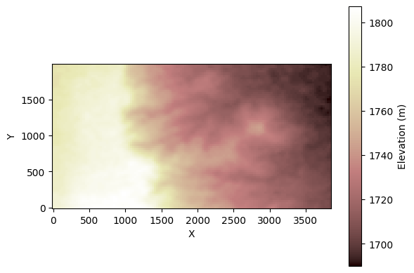
In this example, we read in a small digital elevation model (DEM) from NASADEM for an area on the Colorado high plains (USA) that includes a portion of an escarpment along the west side of a drainage known as West Bijou Creek (see Rengers & Tucker, 2014).

The DEM file is in ESRI Ascii format, but is in a geographic projection, with horizontal units of decimal degrees. To calculate slope gradients properly, we’ll first read the DEM into a Landlab grid object that has this geographic projection. Then we’ll create a second grid with 30 m cell spacing (approximately equal to the NASADEM’s resolution), and copy the elevation field from the geographic DEM. This isn’t a proper projection of course, but it will do for purposes of this example.

# read the DEM
with open("west_bijou_escarpment_snippet.asc") as fp:
    grid_info, data = esri_ascii.lazy_load(fp, name="topographic__elevation", at="node")

grid = RasterModelGrid(grid_info.shape, xy_spacing=30.0)
grid.add_field("topographic__elevation", data, at="node")

array([1789., 1790., 1789., ..., 1691., 1692., 1692.])

grid.imshow(grid.at_node["topographic__elevation"], colorbar_label="Elevation (m)")

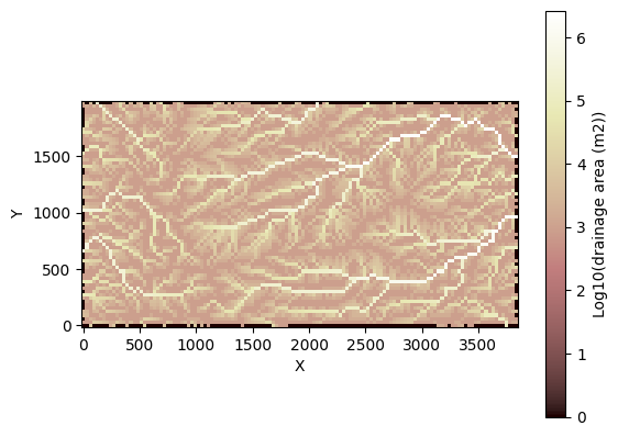
To use DrainageDensity, we need to have drainage directions and areas pre-calculated. We’ll do that with the FlowAccumulator component. We’ll have the component do D8 flow routing (each DEM cell drains to whichever of its 8 neighbors lies in the steepest downslope direction), and fill pits (depressions in the DEM that would otherwise block the flow) using the LakeMapperBarnes component. The latter two arguments below tell the lake mapper to update the flow directions and drainage areas after filling the pits.

fa = FlowAccumulator(
    grid,
    flow_director="FlowDirectorD8",  # use D8 routing
    depression_finder="LakeMapperBarnes",  # pit filler
    method="D8",  # pit filler use D8 too
    redirect_flow_steepest_descent=True,  # re-calculate flow dirs
    reaccumulate_flow=True,  # re-calculate drainagea area
)
fa.run_one_step()  # run the flow accumulator

grid.imshow(
    np.log10(grid.at_node["drainage_area"] + 1.0),  # log10 helps show drainage
    colorbar_label="Log10(drainage area (m2))",
)

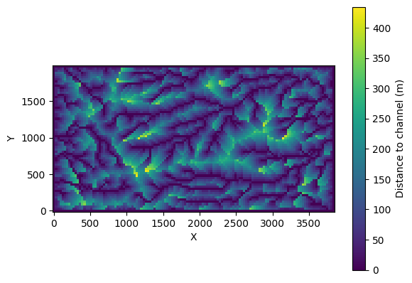
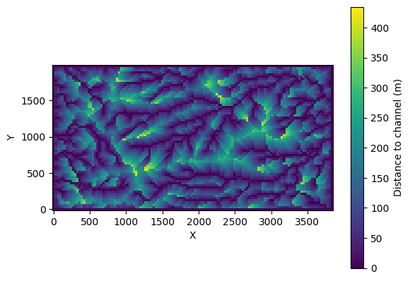
Now run DrainageDensity and display the map of \(L\) values:

dd = DrainageDensity(
    grid,
    area_coefficient=1.0,
    slope_coefficient=1.0,
    area_exponent=1.0,
    slope_exponent=0.0,
    channelization_threshold=2.0e4,
)
ddens = dd.calculate_drainage_density()
grid.imshow(
    grid.at_node["surface_to_channel__minimum_distance"],
    cmap="viridis",
    colorbar_label="Distance to channel (m)",
)
print(f"Drainage density = {ddens} m/m2")

Drainage density = 0.0049234561718207144 m/m2

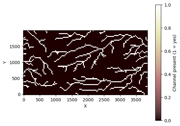
Display the channel mask:

grid.imshow(grid.at_node["channel__mask"], colorbar_label="Channel present (1 = yes)")

Example 2: calculating from an independently derived channel mask

This example demonstrates how to run the component with an independently derived channel mask. For the sake of illustration, we will just use the channel mask from the previous example, in which case the \(L\) field should look identical.

# make a copy of the mask from the previous example
chanmask = grid.at_node["channel__mask"].copy()

# re-make the grid (this will remove all the previously created fields)
grid = RasterModelGrid(grid_info.shape, xy_spacing=30.0)
grid.add_field("topographic__elevation", data, at="node")

array([1789., 1790., 1789., ..., 1691., 1692., 1692.])

# instatiated and run flow accumulator
fa = FlowAccumulator(
    grid,
    flow_director="FlowDirectorD8",  # use D8 routing
    depression_finder="LakeMapperBarnes",  # pit filler
    method="D8",  # pit filler use D8 too
    redirect_flow_steepest_descent=True,  # re-calculate flow dirs
    reaccumulate_flow=True,  # re-calculate drainagea area
)
fa.run_one_step()  # run the flow accumulator

# instantiate and run DrainageDensity component
dd = DrainageDensity(grid, channel__mask=chanmask)
ddens = dd.calculate_drainage_density()

# display distance-to-channel
grid.imshow(
    grid.at_node["surface_to_channel__minimum_distance"],
    cmap="viridis",
    colorbar_label="Distance to channel (m)",
)
print(f"Drainage density = {ddens} m/m2")

Drainage density = 0.004817280239877275 m/m2

References

Rengers, F. K., & Tucker, G. E. (2014). Analysis and modeling of gully headcut dynamics, North American high plains. Journal of Geophysical Research: Earth Surface, 119(5), 983-1003. https://doi.org/10.1002/2013JF002962

Tucker, G. E., Catani, F., Rinaldo, A., & Bras, R. L. (2001). Statistical analysis of drainage density from digital terrain data. Geomorphology, 36(3-4), 187-202, https://doi.org/10.1016/S0169-555X(00)00056-8.

---

Generated by nbsphinx from a Jupyter notebook.