Note

This page was generated from a jupyter notebook.

The Carbonate Producer component

Overview

This notebook demonstrates the CarbonateProducer Landlab component. The component computes the creation of carbonate rocks, such as carbonate platforms and coral reefs, given a particular bathymetry. The component can be used either to calculate the rate of carbonate production (in terms of a vertical deposition rate), or to progressively add to a field representing carbonate thickness. The model does not distinguish among different types of carbonate material, or species of carbonate-producing organism.

Theory

Carbonate production rate

The CarbonateProducer uses the mathematical model of Bosscher and Schlager (1992), which represents the local carbonate growth rate, \(G(x,y,t)\) (thickness per time) as a function of local water depth. The carbonate production rate is calculated as

\[G(x,y,t) = G_m \tanh \left( I_0 e^{-kd} / I_k \right)\]

where:

• \(G_m\) is the maximum production rate

• \(I_0\) is the surface light intensity

• \(I_k\) is the saturating light intensity

• \(d\) is water depth

• \(k\) is the light extinction coefficient

By default the production rate is zero where \(d<0\), but as noted below the user can invoke an option that allows for carbonate production within the tidal range.

Bosscher and Schlager (1992) suggest plausible values or ranges for these parameters as follows: \(G_m\) = 0.010 to 0.015 m/y, \(I_0\) = 2,000 to 2,250 micro Einsteins per square meter per second in the tropics, \(I_k\) = 50 to 450 micro Einsteins per square meter per second, and \(k\) = 0.04 to 0.16 m\(^{-1}\) (corresponding to a decay depth of 6.25 to 16 m).

Smoothing near sea level using tidal range

The default form of the model involves a mathematical discontinuity at zero water depth. The user has the option of smoothing out this discontinuity by passing a positive value for the tidal_range parameter. If this parameter is given, the growth function is modified as follows:

\[G' = H(d) G\]

where \(G\) is the growth rate calculated by the growth function shown above, and \(H(d)\) is a smoothed Heaviside step function of local water depth that is defined as:

\[\begin{split}H(d) = \begin{cases} \frac{1}{1 + \exp(-2 / R_t d)} & \text{if } d > -2R_t \\ 0 & \text{otherwise.} \end{cases}\end{split}\]

Essentially, the \(H(d)\) function allows a limited amount of growth above mean sea level, while reducing the growth rate somewhat within the tidal zone.

Numerical methods

The component’s calc_carbonate_production_rate method can be used to return the current rate of production given the water depths (calculated by subtracting the topographic__elevation node field from the sea_level__elevation grid field). In this case, no numerical methods are needed. This approach might be useful, for example, when modeling simultaneous carbonate and siliciclastic sedimentation, and the user wishes to generate depositional layers that contain some fractional amount of both.

Alternatively, the user can calculate the accumulation of carbonate thickness (in node field carbonate_thickness) by calling either produce_carbonate or run_one_step (the latter simply calls the former). In this case, simple forward Euler differencing is used to add to carbonate thickness, \(C\), via

\[C_i^{k+1} = C_i^k + G_i^k \Delta t\]

where \(i\) refers to node number and \(k\) to time-step number, and \(\Delta t\) is the duration of the time step (passed as an argument to produce_carbonate or run_one_step).

import numpy as np

from landlab import RasterModelGrid
from landlab.components import CarbonateProducer
from landlab.plot import plot_layers

Matplotlib is building the font cache; this may take a moment.

Information about the component

Passing the class name to the help function returns descriptions of the various methods and parameters:

help(CarbonateProducer)

Help on class CarbonateProducer in module landlab.components.carbonate.carbonate_producer:

class CarbonateProducer(landlab.core.model_component.Component)
 |  CarbonateProducer(grid, max_carbonate_production_rate=0.01, extinction_coefficient=0.1, surface_light=2000.0, saturating_light=400.0, tidal_range=0.0)
 |
 |  Calculate marine carbonate production and deposition.
 |
 |  Uses the growth-rate of Bosscher and Schlager (1992), which represents the
 |  vertical growth rate :math:`G` as:
 |
 |  ..math::
 |
 |      G = G_m         anh (I_0 e^{-kz} / I_k)
 |
 |  where :math:`G_m` is the maximum growth rate, :math:`I_0` is the surface
 |  light intensity, :math:`I_k` is the saturating light intensity, :math:`z` is
 |  water depth, and :math:`k` is the light extinction coefficient.
 |
 |  Bosscher and Schlager (1992) suggest plausible values or ranges for these
 |  parameters as follows: :math:`G_m` = 10 to 15 mm/y, :math:`I_0` = 2,000 to
 |  2,250 micro Einsteins per square meter per second in the tropics, :math:`I_k`
 |  = 50 to 450 micro Einsteins per square meter per second, and :math:`k` =
 |  0.04 to 0.16 m:math:`^{-1}` (corresponding to a decay depth of 6.25 to 16 m).
 |  The default values used in this component are based on these estimates.
 |
 |  Examples
 |  --------
 |  >>> from landlab import RasterModelGrid
 |  >>> from landlab.components import CarbonateProducer
 |  >>> grid = RasterModelGrid((3, 3))
 |  >>> elev = grid.add_zeros("topographic__elevation", at="node")
 |  >>> sealevel = grid.add_field("sea_level__elevation", 0.0, at="grid")
 |  >>> elev[:] = -1.0
 |  >>> cp = CarbonateProducer(grid)
 |  >>> np.round(cp.calc_carbonate_production_rate()[4], 2)
 |  0.01
 |  >>> elev[:] = -40.0
 |  >>> np.round(cp.calc_carbonate_production_rate()[4], 5)
 |  0.00091
 |  >>> cp.sea_level = -39.0
 |  >>> np.round(cp.calc_carbonate_production_rate()[4], 2)
 |  0.01
 |  >>> thickness = cp.produce_carbonate(10.0)
 |  >>> np.round(10 * grid.at_node["carbonate_thickness"][4])
 |  1.0
 |  >>> thickness is grid.at_node["carbonate_thickness"]
 |  True
 |  >>> cp.run_one_step(10.0)
 |  >>> np.round(10 * thickness[4])
 |  2.0
 |
 |  References
 |  ----------
 |  Bosscher, H., & Schlager, W. (1992). Computer simulation of reef growth.
 |  Sedimentology, 39(3), 503-512.
 |
 |  Method resolution order:
 |      CarbonateProducer
 |      landlab.core.model_component.Component
 |      builtins.object
 |
 |  Methods defined here:
 |
 |  __init__(self, grid, max_carbonate_production_rate=0.01, extinction_coefficient=0.1, surface_light=2000.0, saturating_light=400.0, tidal_range=0.0)
 |      Parameters
 |      ----------
 |      grid: ModelGrid (RasterModelGrid, HexModelGrid, etc.)
 |          A landlab grid object.
 |      max_carbonate_production_rate: float (default 0.01 m/y)
 |          Maximum rate of carbonate production, in m thickness per year
 |      extinction_coefficient: float (default 0.1 m^-1)
 |          Coefficient of light extinction in water column
 |      surface_light: float (default 2000.0 micro Einstein per m2 per s)
 |          Light intensity (photosynthetic photon flux density) at sea surface.
 |      saturating_light: float (default 400.0 micro Einstein per m2 per s)
 |          Saturating light intensity (photosynthetic photon flux density)
 |      tidal_range: float (default zero)
 |          Tidal range used to smooth growth rate when surface is near mean
 |          sea level.
 |
 |  calc_carbonate_production_rate(self)
 |      Update carbonate production rate and store in field.
 |
 |      Returns
 |      -------
 |      float array x number of grid nodes
 |          Reference to updated carbonate_production_rate field
 |
 |  produce_carbonate(self, dt)
 |      Grow carbonate for one time step & add to carbonate thickness field.
 |
 |      If optional carbonate_thickness field does not already exist, this
 |      function creates it and initializes all values to zero.
 |
 |      Returns
 |      -------
 |      float array x number of grid nodes
 |          Reference to updated carbonate_thickness field
 |
 |  run_one_step(self, dt)
 |      Advance by one time step.
 |
 |      Simply calls the produce_carbonate() function.
 |
 |      Parameters
 |      ----------
 |      dt : float
 |          Time step duration (normally in years)
 |
 |  ----------------------------------------------------------------------
 |  Data descriptors defined here:
 |
 |  extinction_coefficient
 |
 |  max_carbonate_production_rate
 |
 |  saturating_light
 |
 |  sea_level
 |
 |  surface_light
 |
 |  tidal_range
 |
 |  ----------------------------------------------------------------------
 |  Methods inherited from landlab.core.model_component.Component:
 |
 |  initialize_optional_output_fields(self)
 |      Create fields for a component based on its optional field outputs,
 |      if declared in _optional_var_names.
 |
 |      This method will create new fields (without overwrite) for any
 |      fields output by the component as optional. New fields are
 |      initialized to zero. New fields are created as arrays of floats,
 |      unless the component also contains the specifying property
 |      _var_type.
 |
 |  initialize_output_fields(self, values_per_element=None)
 |      Create fields for a component based on its input and output var
 |      names.
 |
 |      This method will create new fields (without overwrite) for any fields
 |      output by, but not supplied to, the component. New fields are
 |      initialized to zero. Ignores optional fields. New fields are created as
 |      arrays of floats, unless the component specifies the variable type.
 |
 |      Parameters
 |      ----------
 |      values_per_element: int (optional)
 |          On occasion, it is necessary to create a field that is of size
 |          (n_grid_elements, values_per_element) instead of the default size
 |          (n_grid_elements,). Use this keyword argument to acomplish this
 |          task.
 |
 |  ----------------------------------------------------------------------
 |  Class methods inherited from landlab.core.model_component.Component:
 |
 |  from_path(grid, path)
 |      Create a component from an input file.
 |
 |      Parameters
 |      ----------
 |      grid : ModelGrid
 |          A landlab grid.
 |      path : str or file_like
 |          Path to a parameter file, contents of a parameter file, or
 |          a file-like object.
 |
 |      Returns
 |      -------
 |      Component
 |          A newly-created component.
 |
 |  var_definition(name)
 |      Get a description of a particular field.
 |
 |      Parameters
 |      ----------
 |      name : str
 |          A field name.
 |
 |      Returns
 |      -------
 |      tuple of (*name*, *description*)
 |          A description of each field.
 |
 |  var_help(name)
 |      Print a help message for a particular field.
 |
 |      Parameters
 |      ----------
 |      name : str
 |          A field name.
 |
 |  var_loc(name)
 |      Location where a particular variable is defined.
 |
 |      Parameters
 |      ----------
 |      name : str
 |          A field name.
 |
 |      Returns
 |      -------
 |      str
 |          The location ('node', 'link', etc.) where a variable is defined.
 |
 |  var_type(name)
 |      Returns the dtype of a field (float, int, bool, str...).
 |
 |      Parameters
 |      ----------
 |      name : str
 |          A field name.
 |
 |      Returns
 |      -------
 |      dtype
 |          The dtype of the field.
 |
 |  var_units(name)
 |      Get the units of a particular field.
 |
 |      Parameters
 |      ----------
 |      name : str
 |          A field name.
 |
 |      Returns
 |      -------
 |      str
 |          Units for the given field.
 |
 |  ----------------------------------------------------------------------
 |  Static methods inherited from landlab.core.model_component.Component:
 |
 |  __new__(cls, *args, **kwds)
 |      Create and return a new object.  See help(type) for accurate signature.
 |
 |  ----------------------------------------------------------------------
 |  Readonly properties inherited from landlab.core.model_component.Component:
 |
 |  cite_as
 |      Citation information for component.
 |
 |      Return required software citation, if any. An empty string indicates
 |      that no citations other than the standard Landlab package citations are
 |      needed for the component.
 |
 |      Citations are provided in BibTeX format.
 |
 |      Returns
 |      -------
 |      cite_as
 |
 |  coords
 |      Return the coordinates of nodes on grid attached to the
 |      component.
 |
 |  definitions
 |      Get a description of each field.
 |
 |      Returns
 |      -------
 |      tuple of (*name*, *description*)
 |          A description of each field.
 |
 |  grid
 |      Return the grid attached to the component.
 |
 |  input_var_names
 |      Names of fields that are used by the component.
 |
 |      Returns
 |      -------
 |      tuple of str
 |          Tuple of field names.
 |
 |  name
 |      Name of the component.
 |
 |      Returns
 |      -------
 |      str
 |          Component name.
 |
 |  optional_var_names
 |      Names of fields that are optionally provided by the component, if
 |      any.
 |
 |      Returns
 |      -------
 |      tuple of str
 |          Tuple of field names.
 |
 |  output_var_names
 |      Names of fields that are provided by the component.
 |
 |      Returns
 |      -------
 |      tuple of str
 |          Tuple of field names.
 |
 |  shape
 |      Return the grid shape attached to the component, if defined.
 |
 |  unit_agnostic
 |      Whether the component is unit agnostic.
 |
 |      If True, then the component is unit agnostic. Under this condition a
 |      user must still provide consistent units across all input arguments,
 |      keyword arguments, and fields. However, when ``unit_agnostic`` is True
 |      the units specified can be interpreted as dimensions.
 |
 |      When False, then the component requires inputs in the specified units.
 |
 |      Returns
 |      -------
 |      bool
 |
 |  units
 |      Get the units for all field values.
 |
 |      Returns
 |      -------
 |      tuple or str
 |          Units for each field.
 |
 |  var_mapping
 |      Location where variables are defined.
 |
 |      Returns
 |      -------
 |      tuple of (name, location)
 |          Tuple of variable name and location ('node', 'link', etc.) pairs.
 |
 |  ----------------------------------------------------------------------
 |  Data descriptors inherited from landlab.core.model_component.Component:
 |
 |  __dict__
 |      dictionary for instance variables
 |
 |  __weakref__
 |      list of weak references to the object
 |
 |  current_time
 |      Current time.
 |
 |      Some components may keep track of the current time. In this case, the
 |      ``current_time`` attribute is incremented. Otherwise it is set to None.
 |
 |      Returns
 |      -------
 |      current_time

Examples

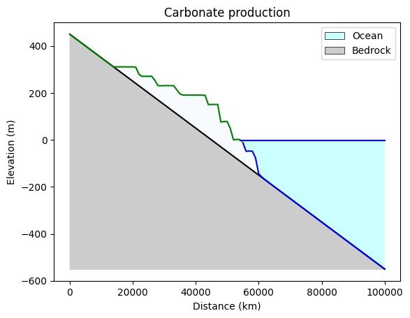
Example 1: carbonate growth on a rising continental margin under sinusoidal sea-level variation

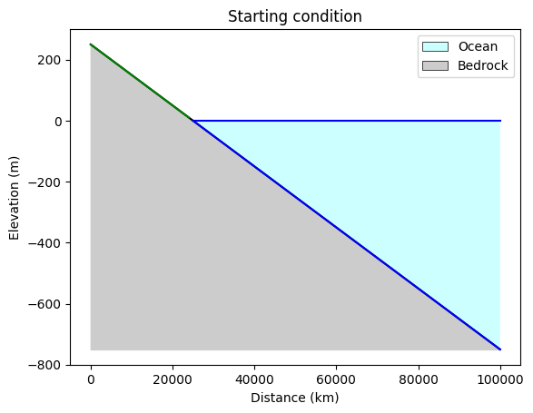
In this example, we consider a sloping ramp that rises tectonically while sea level oscillates.

# Parameters and settings
nrows = 3  # number of grid rows
ncols = 101  # number of grid columns
dx = 1000.0  # node spacing, m
sl_range = 120.0  # range of sea-level variation, m
sl_period = 40000.0  # period of sea-level variation, y
run_duration = 200000.0  # duration of run, y
dt = 100.0  # time-step size, y
initial_shoreline_pos = 25000.0  # starting position of the shoreline, m
topo_slope = 0.01  # initial slope of the topography/bathymetry, m/m
uplift_rate = 0.001  # rate of tectonic uplift, m/y
plot_ylims = [-1000.0, 1000.0]

# Derived parameters
num_steps = int(run_duration / dt)
sin_fac = 2.0 * np.pi / sl_period  # factor for sine calculation of sea-level
middle_row = np.arange(ncols, 2 * ncols, dtype=int)

# Grid and fields
#
# Create a grid object
grid = RasterModelGrid((nrows, ncols), xy_spacing=dx)

# Create sea level field (a scalar, a.k.a. a "grid field")
sea_level = grid.add_field("sea_level__elevation", 0.0, at="grid")

# Create elevation field and initialize as a sloping ramp
bedrock_elevation = topo_slope * (initial_shoreline_pos - grid.x_of_node)
elev = grid.add_field("topographic__elevation", bedrock_elevation.copy(), at="node")
# elev[:] = topo_slope * (initial_shoreline_pos - grid.x_of_node)

# Remember IDs of middle row of nodes, for plotting
middle_row = np.arange(ncols, 2 * ncols, dtype=int)

plot_layers(
    bedrock_elevation[middle_row],
    x=grid.x_of_node[middle_row],
    sea_level=grid.at_grid["sea_level__elevation"],
    x_label="Distance (km)",
    y_label="Elevation (m)",
    title="Starting condition",
    legend_location="upper right",
)

# Instantiate component
cp = CarbonateProducer(grid)

# RUN
for i in range(num_steps):
    cp.sea_level = sl_range * np.sin(sin_fac * i * dt)
    cp.produce_carbonate(dt)
    elev[:] += uplift_rate * dt

plot_layers(
    [
        elev[middle_row] - grid.at_node["carbonate_thickness"][middle_row],
        elev[middle_row],
    ],
    x=grid.x_of_node[middle_row],
    sea_level=grid.at_grid["sea_level__elevation"],
    color_layer="Blues",
    x_label="Distance (km)",
    y_label="Elevation (m)",
    title="Carbonate production",
    legend_location="upper right",
)

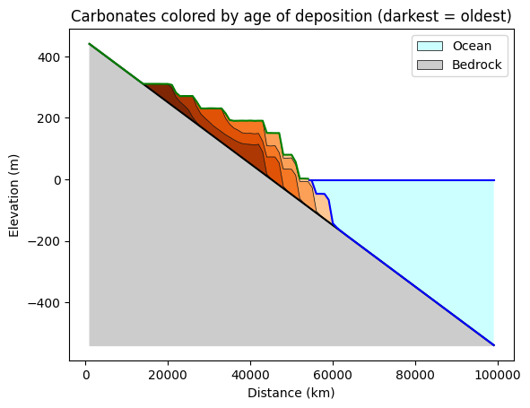
Example 2: tracking stratigraphy

Here we repeat the same example, except this time we use Landlab’s MaterialLayers class to track stratigraphy.

# Track carbonate strata in time bundles of the below duration:
layer_time_interval = 20000.0

# Derived parameters and miscellaneous
next_layer_time = layer_time_interval
time_period_index = 0
time_period = "0 to " + str(int(layer_time_interval) // 1000) + " ky"

# Grid and fields
grid = RasterModelGrid((nrows, ncols), xy_spacing=dx)
sea_level = grid.add_field("sea_level__elevation", 0.0, at="grid")
base_elev = grid.add_zeros("basement__elevation", at="node")
base_elev[:] = topo_slope * (initial_shoreline_pos - grid.x_of_node)
elev = grid.add_zeros("topographic__elevation", at="node")
middle_row = np.arange(ncols, 2 * ncols, dtype=int)
middle_row_cells = np.arange(0, ncols - 2, dtype=int)
carbo_thickness = grid.add_zeros("carbonate_thickness", at="node")
prior_carbo_thickness = np.zeros(grid.number_of_nodes)

# Instantiate component
cp = CarbonateProducer(grid)

# RUN
for i in range(num_steps):
    cp.sea_level = sl_range * np.sin(sin_fac * i * dt)
    cp.produce_carbonate(dt)
    base_elev[:] += uplift_rate * dt
    elev[:] = base_elev + carbo_thickness
    if (i + 1) * dt >= next_layer_time:
        time_period_index += 1
        next_layer_time += layer_time_interval
    added_thickness = np.maximum(
        carbo_thickness - prior_carbo_thickness, 0.00001
    )  # force a tiny bit of depo to keep layers consistent
    prior_carbo_thickness[:] = carbo_thickness
    # grid.material_layers.add(added_thickness[grid.node_at_cell], age=time_period_index)
    grid.event_layers.add(added_thickness[grid.node_at_cell], age=time_period_index)

First get the layers we want to plot. In this case, plot the bottom and top layers as well as layers that correspond to sea level high stands. For the sinusoidal sea level curve we used, high stands occur every 400 time steps, with the first one being at time step 100.

layers = (
    np.vstack(
        [
            grid.event_layers.z[0],
            grid.event_layers.z[100::400],
            grid.event_layers.z[-1],
        ]
    )
    + grid.at_node["basement__elevation"][grid.node_at_cell]
)

plot_layers(
    layers,
    x=grid.x_of_node[grid.node_at_cell],
    sea_level=grid.at_grid["sea_level__elevation"],
    color_layer="Oranges_r",
    legend_location="upper right",
    x_label="Distance (km)",
    y_label="Elevation (m)",
    title="Carbonates colored by age of deposition (darkest = oldest)",
)

References

Bosscher, H., & Schlager, W. (1992). Computer simulation of reef growth. Sedimentology, 39(3), 503-512.

Galewsky, J. (1998). The dynamics of foreland basin carbonate platforms: tectonic and eustatic controls. Basin Research, 10(4), 409-416.

---

Generated by nbsphinx from a Jupyter notebook.