Note

This page was generated from a jupyter notebook.

Introduction to the ErosionDeposition component

This tutorial introduces the ErosionDeposition component, which simulates erosion and deposition in a river network over long time scales.

Theory and Overview

ErosionDeposition models fluvial processes using the approach described by Davy and Lague (2009). The basic goal is to calculate rates of erosion or deposition in the various branches of a river network that is embedded in a gridded landscape (see, e.g., Tucker and Hancock, 2010). The literature has a number of different approaches to this problem. Some models assume transport-limited conditions, such that erosion or deposition result from local imbalances in sediment transport capacity (see, e.g., Willgoose, 2018). Some assume detachment-limited conditions, such that any eroded sediment is entirely removed (e.g., Howard, 1994; Whipple and Tucker, 1999; Tucker and Whipple, 2002). Still others allow for both erosion of detachment-resistant material (bedrock or cohesive sediments), and re-deposition of that material. The Davy-Lague approach falls in the latter category, and is similar to the approach used in some shorter-term morphodynamic models as well as agricultural soil erosion models. The basic idea involves conservation of sediment mass in the water column of a river. One calculates the rate of entrainment of sediment from the bed into the water as a function of discharge and local slope. The bed also accumulates sediment that settles out from the water column, at a rate that depends on sediment concentration (treated as the ratio of sediment flux to water discharge) and a settling-velocity parameter.

The theory behind using this kind of dual erosion-deposition approach in the context of fluvial landscape evolution is described by Davy and Lague (2009). Tucker and Hancock (2010) provide a review of landscape evolution modeling that compares this with other approaches to fluvial erosion/deposition theory. The equations used in the Landlab ErosionDeposition component are described by Barnhart et al. (2019) as part of the terrainBento collection of Landlab-based landscape evolution models, which includes models that use ErosionDeposition.

import copy

import matplotlib as mpl
import matplotlib.pyplot as plt
import numpy as np

from landlab import HexModelGrid
from landlab.components import ErosionDeposition, FlowAccumulator
from landlab.plot import imshow_grid

Look at the top-level internal documentation for the ErosionDeposition component:

print(ErosionDeposition.__doc__)

Erosion-Deposition model in the style of Davy and Lague (2009).

    Erosion-Deposition model in the style of Davy and Lague (2009). It uses a
    mass balance approach across the total sediment mass both in the bed and
    in transport coupled with explicit representation of the sediment
    transport lengthscale (the "xi-q" model) to derive a range of erosional
    and depositional responses in river channels.

    This implementation is close to the Davy & Lague scheme, with a few
    deviations:

    * A fraction of the eroded sediment is permitted to enter the wash load,
      and lost to the mass balance (``F_f``).
    * Here an incision threshold ``omega`` is permitted, where it was not by Davy &
      Lague. It is implemented with an exponentially smoothed form to prevent
      discontinuities in the parameter space. See the
      :py:class:`~landlab.components.StreamPowerSmoothThresholdEroder`
      for more documentation.
    * This component uses an "effective" settling velocity, ``v_s``, as one of its
      inputs. This parameter is simply equal to Davy & Lague's ``d_star * V``
      dimensionless number.

    Erosion of the bed follows a stream power formulation, i.e.::

        E = K * q**m_sp * S**n_sp - omega

    Note that the transition between transport-limited and detachment-limited
    behavior is controlled by the dimensionless ratio (``v_s / r``) where ``r`` is the
    runoff ratio (``Q=Ar``). ``r`` can be changed in the flow accumulation component
    but is not changed within ErosionDeposition. Because the runoff ratio ``r``
    is not changed within the ErosionDeposition component, ``v_s`` becomes the
    parameter that fundamentally controls response style. Very small ``v_s`` will
    lead to a detachment-limited response style, very large ``v_s`` will lead to a
    transport-limited response style. ``v_s == 1`` means equal contributions from
    transport and erosion, and a hybrid response as described by Davy & Lague.

    Unlike other some other fluvial erosion componets in Landlab, in this
    component (and :py:class:`~landlab.components.SPACE`) no erosion occurs
    in depressions or in areas with adverse slopes. There is no ability to
    pass a keyword argument ``erode_flooded_nodes``.

    If depressions are handled (as indicated by the presence of the field
    ``"flood_status_code"`` at nodes), then deposition occurs throughout the
    depression and sediment is passed out of the depression. Where pits are
    encountered, then all sediment is deposited at that node only.

    Component written by C. Shobe, K. Barnhart, and G. Tucker.

    References
    ----------
    **Required Software Citation(s) Specific to this Component**

    Barnhart, K., Glade, R., Shobe, C., Tucker, G. (2019). Terrainbento 1.0: a
    Python package for multi-model analysis in long-term drainage basin
    evolution. Geoscientific Model Development  12(4), 1267--1297.
    https://dx.doi.org/10.5194/gmd-12-1267-2019

    **Additional References**

    Davy, P., Lague, D. (2009). Fluvial erosion/transport equation of landscape
    evolution models revisited Journal of Geophysical Research  114(F3),
    F03007. https://dx.doi.org/10.1029/2008jf001146

    Examples
    ---------
    >>> import numpy as np
    >>> from landlab import RasterModelGrid
    >>> from landlab.components import FlowAccumulator
    >>> from landlab.components import DepressionFinderAndRouter
    >>> from landlab.components import ErosionDeposition
    >>> from landlab.components import FastscapeEroder
    >>> np.random.seed(seed=5000)

    Define grid and initial topography:

    * 5x5 grid with baselevel in the lower left corner
    * All other boundary nodes closed
    * Initial topography is plane tilted up to the upper right + noise

    >>> nr = 5
    >>> nc = 5
    >>> dx = 10
    >>> grid = RasterModelGrid((nr, nc), xy_spacing=10.0)
    >>> grid.at_node["topographic__elevation"] = (
    ...     grid.node_y / 10
    ...     + grid.node_x / 10
    ...     + np.random.rand(grid.number_of_nodes) / 10
    ... )
    >>> grid.set_closed_boundaries_at_grid_edges(
    ...     bottom_is_closed=True,
    ...     left_is_closed=True,
    ...     right_is_closed=True,
    ...     top_is_closed=True,
    ... )
    >>> grid.set_watershed_boundary_condition_outlet_id(
    ...     0, grid.at_node["topographic__elevation"], -9999.0
    ... )
    >>> fsc_dt = 100.0
    >>> ed_dt = 1.0

    Check initial topography

    >>> grid.at_node["topographic__elevation"].reshape(grid.shape)
    array([[0.02290479, 1.03606698, 2.0727653 , 3.01126678, 4.06077707],
           [1.08157495, 2.09812694, 3.00637448, 4.07999597, 5.00969486],
           [2.04008677, 3.06621577, 4.09655859, 5.04809001, 6.02641123],
           [3.05874171, 4.00585786, 5.0595697 , 6.04425233, 7.05334077],
           [4.05922478, 5.0409473 , 6.07035008, 7.0038935 , 8.01034357]])

    Instantiate Fastscape eroder, flow router, and depression finder

    >>> fr = FlowAccumulator(grid, flow_director="D8")
    >>> df = DepressionFinderAndRouter(grid)
    >>> fsc = FastscapeEroder(grid, K_sp=0.001, m_sp=0.5, n_sp=1)

    Burn in an initial drainage network using the Fastscape eroder:

    >>> for _ in range(100):
    ...     fr.run_one_step()
    ...     df.map_depressions()
    ...     flooded = np.where(df.flood_status == 3)[0]
    ...     fsc.run_one_step(dt=fsc_dt)
    ...     grid.at_node["topographic__elevation"][0] -= 0.001  # uplift
    ...

    Instantiate the E/D component:

    >>> ed = ErosionDeposition(
    ...     grid, K=0.00001, v_s=0.001, m_sp=0.5, n_sp=1.0, sp_crit=0
    ... )

    Now run the E/D component for 2000 short timesteps:

    >>> for _ in range(2000):  # E/D component loop
    ...     fr.run_one_step()
    ...     df.map_depressions()
    ...     ed.run_one_step(dt=ed_dt)
    ...     grid.at_node["topographic__elevation"][0] -= 2e-4 * ed_dt
    ...

    Now we test to see if topography is right:

    >>> np.around(grid.at_node["topographic__elevation"], decimals=3).reshape(
    ...     grid.shape
    ... )
    array([[-0.477,  1.036,  2.073,  3.011,  4.061],
           [ 1.082, -0.08 , -0.065, -0.054,  5.01 ],
           [ 2.04 , -0.065, -0.065, -0.053,  6.026],
           [ 3.059, -0.054, -0.053, -0.035,  7.053],
           [ 4.059,  5.041,  6.07 ,  7.004,  8.01 ]])

The __init__ docstring lists the parameters for this component:

print(ErosionDeposition.__init__.__doc__)

Initialize the ErosionDeposition model.

        Parameters
        ----------
        grid : ModelGrid
            Landlab ModelGrid object
        K : str or array_like, optional
            Erodibility for substrate (units vary).
        v_s : str or array_like, optional
            Effective settling velocity for chosen grain size metric [L/T].
        m_sp : float, optional
            Discharge exponent (units vary)
        n_sp : float, optional
            Slope exponent (units vary)
        sp_crit : str or array_like, optional
            Critical stream power to erode substrate [E/(TL^2)]
        F_f : float, optional
            Fraction of eroded material that turns into "fines" that do not
            contribute to (coarse) sediment load. Defaults to zero.
        discharge_field : str or array_like, optional
            Discharge [L^2/T]. The default is to use the grid field
            'surface_water__discharge', which is simply drainage area
            multiplied by the default rainfall rate (1 m/yr). To use custom
            spatially/temporally varying rainfall, use 'water__unit_flux_in'
            to specify water input to the FlowAccumulator.
        solver : {"basic", "adaptive"}, optional
            Solver to use. Options at present include:

            1. "basic" (default): explicit forward-time extrapolation.
               Simple but will become unstable if time step is too large.
            2. "adaptive": adaptive time-step solver that estimates a
               stable step size based on the shortest time to "flattening"
               among all upstream-downstream node pairs.

Set some parameters:

# Parameters
nrows = 41
ncols = 41
dx = 100.0
K = 0.0001  # erodibility coefficient, 1/yr
m_sp = 0.5  # exponent on drainage area or discharge, -
n_sp = 1.0  # exponent on slope, -
sp_crit = 0.0  # erosion threshold
v_s = 100.0  # settling velocity parameter (dimensionless if drainage area is used instead of discharge)
F_f = 0.5  # fraction of fines generated during bed erosion
initial_elevation = (
    200.0  # starting elevation of an "uplifted block" (rapid baselevel drop), m
)

run_duration = 120000.0  # duration of run, yr
dt = 100.0  # time-step duration, yr
plot_every = 40000.0  # time interval for plotting, yr

# Derived parameters
nsteps = int(run_duration / dt)
next_plot = plot_every

# set up colormap
cmap = copy.copy(mpl.colormaps["pink"])

Create a grid with one side open:

mg = HexModelGrid(
    (nrows, ncols), spacing=dx, node_layout="rect", orientation="vertical"
)
z = mg.add_zeros("topographic__elevation", at="node")
# add some roughness, as this lets "natural" channel planforms arise
np.random.seed(0)
initial_roughness = np.random.rand(z.size)
z[:] += initial_roughness
z[mg.core_nodes] += initial_elevation
z[mg.boundary_nodes] = 0.0

# close off boundaries on 3 sides
is_closed_boundary = np.logical_and(
    mg.status_at_node != mg.BC_NODE_IS_CORE,
    mg.x_of_node < (np.amax(mg.x_of_node) - 0.5 * dx),
)
mg.status_at_node[is_closed_boundary] = mg.BC_NODE_IS_CLOSED

Instantiate components:

fr = FlowAccumulator(mg, depression_finder="DepressionFinderAndRouter")
ed = ErosionDeposition(
    mg,
    K=K,
    m_sp=m_sp,
    n_sp=n_sp,
    sp_crit=sp_crit,
    v_s=v_s,
    F_f=F_f,
    solver="adaptive",  # use the adaptive time stepper, which is slightly faster
)

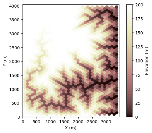
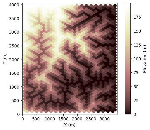
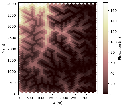
Run the model in a loop to evolve topography on the uplifted block:

for i in range(1, nsteps + 1):
    # route flow
    fr.run_one_step()  # run_one_step isn't time sensitive, so it doesn't take dt as input

    # do some erosion/deposition
    ed.run_one_step(dt)

    if i * dt >= next_plot:
        plt.figure()
        imshow_grid(
            mg,
            "topographic__elevation",
            grid_units=["m", "m"],
            var_name="Elevation (m)",
            cmap=cmap,
        )
        next_plot += plot_every

References

Barnhart, K. R., Glade, R. C., Shobe, C. M., & Tucker, G. E. (2019). Terrainbento 1.0: a Python package for multi-model analysis in long-term drainage basin evolution. Geoscientific Model Development, 12(4), 1267-1297.

Davy, P., & Lague, D. (2009). Fluvial erosion/transport equation of landscape evolution models revisited. Journal of Geophysical Research: Earth Surface, 114(F3).

Howard, A. D. (1994). A detachment‐limited model of drainage basin evolution. Water resources research, 30(7), 2261-2285.

Tucker, G. E., & Hancock, G. R. (2010). Modelling landscape evolution. Earth Surface Processes and Landforms, 35(1), 28-50.

Tucker, G. E., & Whipple, K. X. (2002). Topographic outcomes predicted by stream erosion models: Sensitivity analysis and intermodel comparison. Journal of Geophysical Research: Solid Earth, 107(B9), ETG-1.

Whipple, K. X., & Tucker, G. E. (1999). Dynamics of the stream‐power river incision model: Implications for height limits of mountain ranges, landscape response timescales, and research needs. Journal of Geophysical Research: Solid Earth, 104(B8), 17661-17674.

Willgoose, G. (2018). Principles of soilscape and landscape evolution. Cambridge University Press.

---

Generated by nbsphinx from a Jupyter notebook.