Note

This page was generated from a jupyter notebook.

2D Surface Water Flow component

Overview

This notebook demonstrate the usage of the river flow dynamics Landlab component. The component runs a semi-implicit, semi-Lagrangian finite-volume approximation to the depth-averaged 2D shallow-water equations of Casulli and Cheng (1992) and related work.

Theory

The depth-averaged 2D shallow-water equations are the simplification of the Navier-Stokes equations, which correspond to the balance of momentum and mass in the fluid. It is possible to simplify these equations by assuming a well-mixed water column and a small water depth to width ratio, where a vertical integration results in depth-averaged equations. These require boundary conditions at the top and bottom of the water column, which are provided by the wind stress and the Manning-Chezy formula, respectively:

\[\frac{\partial U}{\partial t} + U\frac{\partial U}{\partial x} + V\frac{\partial U}{\partial y} = - g\frac{\partial \eta}{\partial x} + \epsilon\left(\frac{\partial^2 U}{\partial x^2} + \frac{\partial^2 U}{\partial y^2}\right) + \frac{\gamma_T(U_a - U)}{H} - g\frac{\sqrt{U^2 + V^2}}{Cz^2}U + \mathbf{f}V\]

\[\frac{\partial V}{\partial t} + U\frac{\partial V}{\partial x} + V\frac{\partial V}{\partial y} = - g\frac{\partial \eta}{\partial y} + \epsilon\left(\frac{\partial^2 V}{\partial x^2} + \frac{\partial^2 V}{\partial y^2}\right) + \frac{\gamma_T(V_a - V)}{H} - g\frac{\sqrt{U^2 + V^2}}{Cz^2}V + \mathbf{f}U\]

\[\frac{\partial \eta}{\partial t} + \frac{\partial (HU)}{\partial x} + \frac{\partial (HV)}{\partial y} = 0\]

where \(U\) is the water velocity in the \(x\)-direction, \(V\) is the water velocity in the \(y\)-direction, \(H\) is the water depth, \(\eta\) is the water surface elevation, \(Cz\) is the Chezy friction coefficient, and \(t\) is time. For the constants \(g\) is the gravity acceleration, \(\epsilon\) is the horizontal eddy viscosity, \(\mathbf{f}\) is the Coriolis parameter, \(\gamma_T\) is the wind stress coefficient, and \(U_a\) and \(V_a\) are the prescribed wind velocities.

Numerical representation

A semi-implicit, semi-Lagrangian, finite volume numerical approximation represents the depth averaged, 2D shallow-water equations described before. The water surface elevation, \(\eta\), is defined at the center of each computational volume (nodes). Water depth, \(H\), and velocity components, \(U\) and \(V\), are defined at the midpoint of volume faces (links). The finite volume structure provides a control volume representation that is inherently mass conservative.

The combination of a semi-implciit water surface elevation solution and a semi-Lagrangian representation of advection provides the advantages of a stable solution and of time steps that exceed the CFL criterion. In the semi-implicit process, \(\eta\) in the momentum equations, and the velocity divergence in the continuity equation, are treated implicitly. The advective terms in the momentum equations, are discretized explicitly. See the cited literature for more details.

The component

Import the needed libraries:

import matplotlib.pyplot as plt
import numpy as np
from IPython.display import clear_output
from tqdm import trange

from landlab import RasterModelGrid
from landlab.components import RiverFlowDynamics
from landlab.io import esri_ascii

Information about the component

Using the class name as argument for the help function returns descriptions of the various methods and parameters.

help(RiverFlowDynamics)

Help on class RiverFlowDynamics in module landlab.components.river_flow_dynamics.river_flow_dynamics:

class RiverFlowDynamics(landlab.core.model_component.Component)
 |  RiverFlowDynamics(grid, dt=0.01, eddy_viscosity=0.0001, mannings_n=0.012, threshold_depth=0.01, theta=0.5, fixed_entry_nodes=None, fixed_entry_links=None, entry_nodes_h_values=None, entry_links_vel_values=None, pcg_tolerance=1e-05, pcg_max_iterations=None, surface_water__elevation_at_N_1=0.0, surface_water__elevation_at_N_2=0.0, surface_water__velocity_at_N_1=0.0)
 |
 |  Simulate surface fluid flow based on Casulli and Cheng (1992).
 |
 |  This Landlab component simulates surface fluid flow using the approximations of the
 |  2D shallow water equations developed by Casulli and Cheng in 1992. It calculates water
 |  depth and velocity across the raster grid, given a specific input discharge.
 |
 |  References
 |  ----------
 |  **Required Software Citation(s) Specific to this Component**
 |
 |  None Listed
 |
 |  **Additional References**
 |
 |  Casulli, V., Cheng, R.T. (1992). “Semi-implicit finite difference methods for
 |  three-dimensional shallow water flow”. International Journal for Numerical Methods
 |  in Fluids. 15: 629-648.
 |  https://doi.org/10.1002/fld.1650150602
 |
 |  Method resolution order:
 |      RiverFlowDynamics
 |      landlab.core.model_component.Component
 |      builtins.object
 |
 |  Methods defined here:
 |
 |  __init__(self, grid, dt=0.01, eddy_viscosity=0.0001, mannings_n=0.012, threshold_depth=0.01, theta=0.5, fixed_entry_nodes=None, fixed_entry_links=None, entry_nodes_h_values=None, entry_links_vel_values=None, pcg_tolerance=1e-05, pcg_max_iterations=None, surface_water__elevation_at_N_1=0.0, surface_water__elevation_at_N_2=0.0, surface_water__velocity_at_N_1=0.0)
 |      Simulate the vertical-averaged surface fluid flow
 |
 |      Simulate vertical-averaged surface fluid flow using the Casulli and Cheng (1992)
 |      approximations of the 2D shallow water equations. This Landlab component calculates
 |      water depth and velocity across the raster grid based on a given input discharge.
 |
 |      Parameters
 |      ----------
 |      grid : RasterModelGrid
 |          A grid.
 |      dt : float, optional
 |          Time step in seconds. If not provided, it is calculated from the CFL condition.
 |      eddy_viscosity : float, optional
 |          Eddy viscosity coefficient. Default = 1e-4 :math:`m^2 / s`
 |      mannings_n : float or array_like, optional
 |          Manning's roughness coefficient. Default = 0.012 :math:`s / m^1/3`
 |      threshold_depth : float, optional
 |          Threshold at which a cell is considered wet. Default = 0.01 m
 |      theta : float, optional
 |          Degree of 'implicitness' of the solution, ranging between 0.5 and 1.0.
 |          Default: 0.5. When set to 0.5, the approximation is centered in time;
 |          when set to 1.0, it is fully implicit.
 |      fixed_entry_nodes : array_like or None, optional
 |          Node IDs where flow enters the domain (Dirichlet boundary condition).
 |          If not provided, existing water in the domain is not renewed.
 |      fixed_entry_links : array_like or None, optional
 |          Link IDs where flow enters the domain (Dirichlet boundary condition).
 |          If not provided, existing water in the domain is not renewed.
 |      entry_nodes_h_values : array_like, optional
 |          Water depth values at nodes where flow enters the domain
 |          (Dirichlet boundary condition).
 |          If not provided, existing water in the domain is not renewed.
 |      entry_links_vel_values : array_like, optional
 |          Water velocity values at links where flow enters the domain
 |          (Dirichlet boundary condition).
 |          If not provided, existing water in the domain is not renewed.
 |      pcg_tolerance : float, optional
 |          Tolerance for convergence in the Preconditioned Conjugate Gradient
 |          method. Default: 1e-05.
 |      pcg_max_iterations : integer, optional
 |          Maximum number of iterations for the Preconditioned Conjugate Gradient
 |          method. Iteration stops after maxiter steps, even if the specified
 |          tolerance is not achieved. Default: None.
 |      surface_water__elevation_at_N_1: array_like of float, optional
 |          Water surface elevation at nodes at time N-1 [m].
 |      surface_water__elevation_at_N_2: array_like of float, optional
 |          Water surface elevation at nodes at time N-2 [m].
 |      surface_water__velocity_at_N_1: array_like of float, optional
 |          Speed of water flow at links above the surface at time N-1 [m/s].
 |
 |  find_adjacent_links_at_link(self, current_link, objective_links='horizontal')
 |      Get adjacent links to the link.
 |
 |      This function finds the links at right, above, left and below the given link.
 |      Similar purpose to the "adjacent_nodes_at_node" function.
 |      Return the adjacent links in as many rows as given links.
 |      Link IDs are returned as columns in clock-wise order starting from East (E, N, W, S).
 |
 |  find_nearest_link(self, x_coordinates, y_coordinates, objective_links='all')
 |      Link nearest a point.
 |
 |      Find the index to the link nearest the given x, y coordinates.
 |      Returns the indices of the links nearest the given coordinates.
 |
 |  path_line_tracing(self)
 |      " Path line tracing algorithm.
 |
 |      This function implements the semi-analytical path line tracing method
 |      of Pollock (1988).
 |
 |      The semi-analytical path line tracing method was developed for particle
 |      tracking in ground water flow models. The assumption that each directional
 |      velocity component varies linearly in its coordinate directions within
 |      each computational volume or cell underlies the method.
 |      Linear variation allows the derivation of an analytical expression for
 |      the path line of a particle across a volume.
 |
 |      Given an initial point located at each volume faces of the domain, particle
 |      trayectories are traced backwards on time. Then, this function returns
 |      the departure point of the particle at the beginning of the time step.
 |
 |  run_one_step(self)
 |      Calculate water depth and water velocity for a time period dt.
 |
 |  ----------------------------------------------------------------------
 |  Methods inherited from landlab.core.model_component.Component:
 |
 |  initialize_optional_output_fields(self)
 |      Create fields for a component based on its optional field outputs,
 |      if declared in _optional_var_names.
 |
 |      This method will create new fields (without overwrite) for any
 |      fields output by the component as optional. New fields are
 |      initialized to zero. New fields are created as arrays of floats,
 |      unless the component also contains the specifying property
 |      _var_type.
 |
 |  initialize_output_fields(self, values_per_element=None)
 |      Create fields for a component based on its input and output var
 |      names.
 |
 |      This method will create new fields (without overwrite) for any fields
 |      output by, but not supplied to, the component. New fields are
 |      initialized to zero. Ignores optional fields. New fields are created as
 |      arrays of floats, unless the component specifies the variable type.
 |
 |      Parameters
 |      ----------
 |      values_per_element: int (optional)
 |          On occasion, it is necessary to create a field that is of size
 |          (n_grid_elements, values_per_element) instead of the default size
 |          (n_grid_elements,). Use this keyword argument to acomplish this
 |          task.
 |
 |  ----------------------------------------------------------------------
 |  Class methods inherited from landlab.core.model_component.Component:
 |
 |  from_path(grid, path)
 |      Create a component from an input file.
 |
 |      Parameters
 |      ----------
 |      grid : ModelGrid
 |          A landlab grid.
 |      path : str or file_like
 |          Path to a parameter file, contents of a parameter file, or
 |          a file-like object.
 |
 |      Returns
 |      -------
 |      Component
 |          A newly-created component.
 |
 |  var_definition(name)
 |      Get a description of a particular field.
 |
 |      Parameters
 |      ----------
 |      name : str
 |          A field name.
 |
 |      Returns
 |      -------
 |      tuple of (*name*, *description*)
 |          A description of each field.
 |
 |  var_help(name)
 |      Print a help message for a particular field.
 |
 |      Parameters
 |      ----------
 |      name : str
 |          A field name.
 |
 |  var_loc(name)
 |      Location where a particular variable is defined.
 |
 |      Parameters
 |      ----------
 |      name : str
 |          A field name.
 |
 |      Returns
 |      -------
 |      str
 |          The location ('node', 'link', etc.) where a variable is defined.
 |
 |  var_type(name)
 |      Returns the dtype of a field (float, int, bool, str...).
 |
 |      Parameters
 |      ----------
 |      name : str
 |          A field name.
 |
 |      Returns
 |      -------
 |      dtype
 |          The dtype of the field.
 |
 |  var_units(name)
 |      Get the units of a particular field.
 |
 |      Parameters
 |      ----------
 |      name : str
 |          A field name.
 |
 |      Returns
 |      -------
 |      str
 |          Units for the given field.
 |
 |  ----------------------------------------------------------------------
 |  Static methods inherited from landlab.core.model_component.Component:
 |
 |  __new__(cls, *args, **kwds)
 |      Create and return a new object.  See help(type) for accurate signature.
 |
 |  ----------------------------------------------------------------------
 |  Readonly properties inherited from landlab.core.model_component.Component:
 |
 |  cite_as
 |      Citation information for component.
 |
 |      Return required software citation, if any. An empty string indicates
 |      that no citations other than the standard Landlab package citations are
 |      needed for the component.
 |
 |      Citations are provided in BibTeX format.
 |
 |      Returns
 |      -------
 |      cite_as
 |
 |  coords
 |      Return the coordinates of nodes on grid attached to the
 |      component.
 |
 |  definitions
 |      Get a description of each field.
 |
 |      Returns
 |      -------
 |      tuple of (*name*, *description*)
 |          A description of each field.
 |
 |  grid
 |      Return the grid attached to the component.
 |
 |  input_var_names
 |      Names of fields that are used by the component.
 |
 |      Returns
 |      -------
 |      tuple of str
 |          Tuple of field names.
 |
 |  name
 |      Name of the component.
 |
 |      Returns
 |      -------
 |      str
 |          Component name.
 |
 |  optional_var_names
 |      Names of fields that are optionally provided by the component, if
 |      any.
 |
 |      Returns
 |      -------
 |      tuple of str
 |          Tuple of field names.
 |
 |  output_var_names
 |      Names of fields that are provided by the component.
 |
 |      Returns
 |      -------
 |      tuple of str
 |          Tuple of field names.
 |
 |  shape
 |      Return the grid shape attached to the component, if defined.
 |
 |  unit_agnostic
 |      Whether the component is unit agnostic.
 |
 |      If True, then the component is unit agnostic. Under this condition a
 |      user must still provide consistent units across all input arguments,
 |      keyword arguments, and fields. However, when ``unit_agnostic`` is True
 |      the units specified can be interpreted as dimensions.
 |
 |      When False, then the component requires inputs in the specified units.
 |
 |      Returns
 |      -------
 |      bool
 |
 |  units
 |      Get the units for all field values.
 |
 |      Returns
 |      -------
 |      tuple or str
 |          Units for each field.
 |
 |  var_mapping
 |      Location where variables are defined.
 |
 |      Returns
 |      -------
 |      tuple of (name, location)
 |          Tuple of variable name and location ('node', 'link', etc.) pairs.
 |
 |  ----------------------------------------------------------------------
 |  Data descriptors inherited from landlab.core.model_component.Component:
 |
 |  __dict__
 |      dictionary for instance variables
 |
 |  __weakref__
 |      list of weak references to the object
 |
 |  current_time
 |      Current time.
 |
 |      Some components may keep track of the current time. In this case, the
 |      ``current_time`` attribute is incremented. Otherwise it is set to None.
 |
 |      Returns
 |      -------
 |      current_time

Examples

---

Example 1: Flow in a rectangular channel 6.0 m long

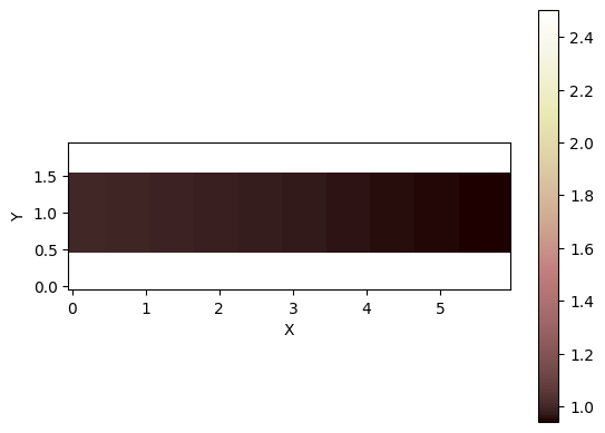
This first basic example illustrates water flowing through a rectangular channel 1.0 \(m\) wide and 6.0 \(m\) long. Our channel is made in concrete, so we choose a Manning’s roughness coefficient equal to 0.012 \(s/m^\frac{1}{3}\), and it has a slope of 0.01 \(m/m\).

We specify some basic parameters such as the grid resolution, time step duration, number of time steps, and the domain dimensions by specifying the number of columns and rows.

# Basic parameters
mannings_n = 0.012  # Manning's roughness coefficient, [s/m^(1/3)]
channel_slope = 0.01  # Channel slope [m/m]

# Simulation parameters
n_timesteps = 1000  # Number of timesteps
dt = 0.1  # Timestep duration, [s]
nrows = 20  # Number of node rows
ncols = 60  # Number of node cols
dx = 0.1  # Node spacing in the x-direction, [m]
dy = 0.1  # Node spacing in the y-direction, [m]

Create the grid:

# Create and set up the grid
grid = RasterModelGrid((nrows, ncols), xy_spacing=(dx, dy))

Create the elevation field and define the topography to represent our rectangular channel:

# The grid represents a basic rectangular channel with slope equal to 0.01 m/m
te = grid.add_field(
    "topographic__elevation", 1.0 - channel_slope * grid.x_of_node, at="node"
)
te[grid.y_of_node > 1.5] = 2.5
te[grid.y_of_node < 0.5] = 2.5

We show a top view of the domain:

# Showing the topography
grid.imshow("topographic__elevation")

The channel is empty at the beginning of the simulation, so we create the fields for the water surface elevation, depth and velocity:

# We establish the initial conditions, which represent an empty channel
h = grid.add_zeros("surface_water__depth", at="node")

# Water velocity is zero in everywhere since there is no water yet
vel = grid.add_zeros("surface_water__velocity", at="link")

# Calculating the initial water surface elevation from water depth and topographic elevation
wse = grid.add_field("surface_water__elevation", te, at="node")

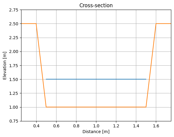
Then, we specify the nodes at which water is entering into the domain, and also the associated links. These are going to be the entry boundary conditions for water depth and velocity. In this case, water flows from left to right at 0.5 \(m\) depth, with a velocity of 0.45 \(m/s\):

# We set fixed boundary conditions, specifying the nodes and links in which the water is flowing into the grid
fixed_entry_nodes = np.array([300, 360, 420, 480, 540, 600, 660, 720, 780, 840, 900])
fixed_entry_links = grid.links_at_node[fixed_entry_nodes][:, 0]

# We set the fixed values in the entry nodes/links
entry_nodes_h_values = np.array([0.5, 0.5, 0.5, 0.5, 0.5, 0.5, 0.5, 0.5, 0.5, 0.5, 0.5])
entry_links_vel_values = np.array(
    [0.45, 0.45, 0.45, 0.45, 0.45, 0.45, 0.45, 0.45, 0.45, 0.45, 0.45]
)

And now we show the boundary condition in the cross-section:

plt.plot(
    grid.y_of_node[fixed_entry_nodes], entry_nodes_h_values + te[fixed_entry_nodes]
)
plt.plot(grid.y_of_node[grid.nodes_at_left_edge], te[grid.nodes_at_left_edge])
plt.title("Cross-section")
plt.xlabel("Distance [m]")
plt.ylabel("Elevation [m]")
plt.axis([0.25, 1.75, 0.75, 2.75])
plt.grid(True)

We construct our component by passing the arguments we defined previously:

# Finally, we run the model and let the water fill our channel
rfd = RiverFlowDynamics(
    grid,
    dt=dt,
    mannings_n=mannings_n,
    fixed_entry_nodes=fixed_entry_nodes,
    fixed_entry_links=fixed_entry_links,
    entry_nodes_h_values=entry_nodes_h_values,
    entry_links_vel_values=entry_links_vel_values,
)

And finally, we run the simulation for 100 timesteps (10 seconds).

# Set the animation frequency to n_timesteps if you
# don't want to plot the water depth
# display_animation_freq = n_timesteps
display_animation_freq = 5

grid.imshow("surface_water__depth", output=True)
for timestep in trange(n_timesteps):
    rfd.run_one_step()

    if timestep % display_animation_freq == 0:
        clear_output(wait=True)  # This will clear the previous image
        grid.imshow("surface_water__depth", output=True)

100%|██████████| 1000/1000 [02:24<00:00,  6.94it/s]

<Figure size 640x480 with 0 Axes>

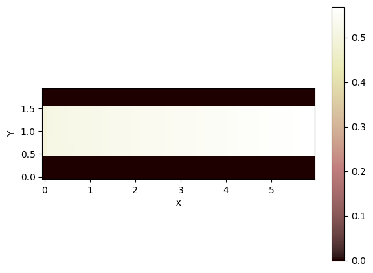
Exploring the water depth results at the latest time:

grid.imshow("surface_water__depth")

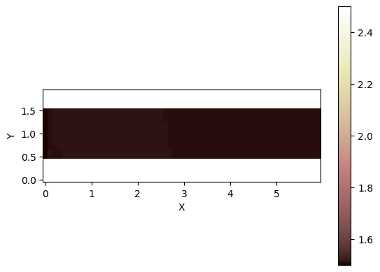
And the water surface elevation:

grid.imshow("surface_water__elevation")

---

Example 2: Surface water flowing over a DEM

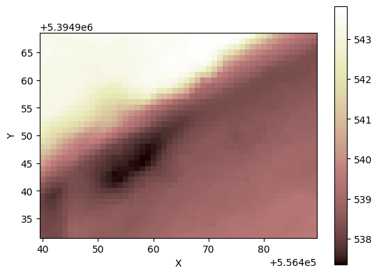
On this case, we will import a digital elevation model (DEM) for a side-channel of the Kootenai River, Idaho, US.

# Getting the grid and some parameters
asc_file = "DEM-kootenai_37x50_1x1.asc"
with open(asc_file) as fp:
    grid = esri_ascii.load(fp, name="topographic__elevation")
te = grid.at_node["topographic__elevation"]

Again, we specify some basic parameters such as the time step number and duration. For simplicity, we will keep our previous Manning’s coefficient. Notice that we already loaded all the required libraries.

# Basic parameters
mannings_n = 0.012  # Manning's roughness coefficient, [s/m^(1/3)]

# Simulation parameters
n_timesteps = 75  # Number of timesteps
dt = 1.0  # Timestep duration, [s]

Let’s see our new topography:

# Showing the topography
grid.imshow("topographic__elevation")

Our side-channel is empty at the beggining of the simulation, so we create the proper fields:

# We establish the initial conditions, which represent an empty channel
h = grid.add_zeros("surface_water__depth", at="node")

# Water velocity is zero in everywhere since there is no water yet
vel = grid.add_zeros("surface_water__velocity", at="link")

# Calculating the initial water surface elevation from water depth and topographic elevation
wse = grid.add_field("surface_water__elevation", te, at="node")

Then, we specify the nodes at which water is entering into the domain, and also the associated links. These are going to be our entry boundary conditions for water depth and velocity. On this case, water flows from right to left:

# We set fixed boundary conditions, specifying the nodes and links in which the water is flowing into the grid
fixed_entry_nodes = grid.nodes_at_right_edge
fixed_entry_links = grid.links_at_node[fixed_entry_nodes][:, 2]

# We set the fixed values in the entry nodes/links
entry_nodes_h_values = np.array(
    [
        0.0,
        0.0,
        0.0,
        0.0,
        0.0,
        0.0,
        0.0,
        0.0,
        0.0,
        0.0,
        0.0,
        0.0,
        0.04998779,
        0.05999756,
        0.03997803,
        0.0,
        0.0,
        0.0,
        0.05999756,
        0.10998535,
        0.12994385,
        0.09997559,
        0.15997314,
        0.23999023,
        0.30999756,
        0.36999512,
        0.45996094,
        0.50994873,
        0.54998779,
        0.59997559,
        0.63995361,
        0.65997314,
        0.65997314,
        0.60998535,
        0.5,
        0.13995361,
        0.0,
    ]
)
entry_links_vel_values = np.array(
    [
        0.0,
        0.0,
        0.0,
        0.0,
        0.0,
        0.0,
        0.0,
        0.0,
        0.0,
        0.0,
        0.0,
        0.0,
        -2.58638018,
        -2.58638018,
        -2.58638018,
        0.0,
        0.0,
        0.0,
        -2.58638018,
        -2.58638018,
        -2.58638018,
        -2.58638018,
        -2.58638018,
        -2.58638018,
        -2.58638018,
        -2.58638018,
        -2.58638018,
        -2.58638018,
        -2.58638018,
        -2.58638018,
        -2.58638018,
        -2.58638018,
        -2.58638018,
        -2.58638018,
        -2.58638018,
        -2.58638018,
        0.0,
    ]
)

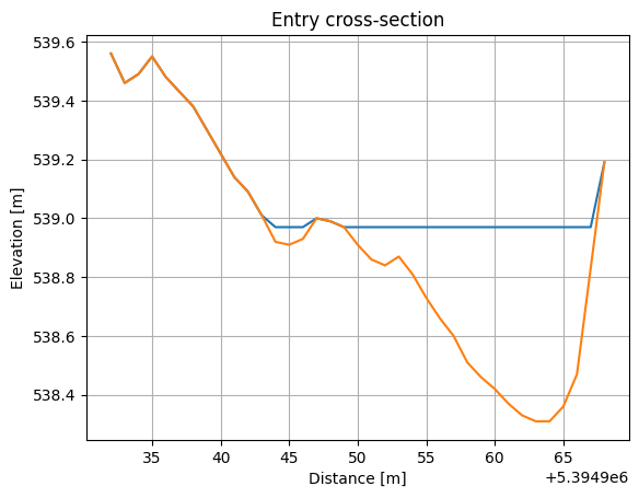
Now we can plot our entry boundary condition in the cross-section:

plt.plot(
    grid.y_of_node[fixed_entry_nodes], entry_nodes_h_values + te[fixed_entry_nodes]
)
plt.plot(grid.y_of_node[grid.nodes_at_right_edge], te[grid.nodes_at_right_edge])
plt.title("Entry cross-section")
plt.xlabel("Distance [m]")
plt.ylabel("Elevation [m]")
plt.grid(True)

Then we create the component by passing the arguments defined previously:

# Finally, we run the model and let the water fill our channel
rfd = RiverFlowDynamics(
    grid,
    dt=dt,
    mannings_n=mannings_n,
    fixed_entry_nodes=fixed_entry_nodes,
    fixed_entry_links=fixed_entry_links,
    entry_nodes_h_values=entry_nodes_h_values,
    entry_links_vel_values=entry_links_vel_values,
)

And we run 75 time steps of 1 \(s\) duration (around 1 minute of computing time):

# Set the animation frequency to n_timesteps if you
# don't want to plot the water depth
# display_animation_freq = n_timesteps
display_animation_freq = 5

grid.imshow("surface_water__depth", output=True)
for timestep in trange(n_timesteps):
    rfd.run_one_step()

    if timestep % display_animation_freq == 0:
        clear_output(wait=True)  # This will clear the previous image
        grid.imshow("surface_water__depth", output=True)

100%|██████████| 75/75 [01:00<00:00,  1.23it/s]

<Figure size 640x480 with 0 Axes>

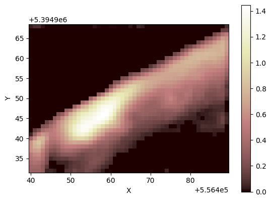
Finally, we can explore the results by plotting the resulting water depth:

grid.imshow("surface_water__depth")

###	And that’s it!
Nic	e work completing this tutorial. You know now how to use the Ri verFlowDynamics Landlab component to run your own simulations :)

Click here for more Landlab tutorials

---

Generated by nbsphinx from a Jupyter notebook.