Note

This page was generated from a jupyter notebook.

Components for modeling overland flow erosion

(G.E. Tucker, July 2021)

There are two related components that calculate erosion resulting from surface-water flow, a.k.a. overland flow: DepthSlopeProductErosion and DetachmentLtdErosion. They were originally created by Jordan Adams to work with the OverlandFlow component, which solves for water depth across the terrain. They are similar to the StreamPowerEroder and FastscapeEroder components in that they calculate erosion resulting from water flow across a topographic surface, but whereas these components require a flow-routing algorithm to create a list of node “receivers”, the DepthSlopeProductErosion and DetachmentLtdErosion components only require a user-identified slope field together with an at-node depth or discharge field (respectively).

DepthSlopeProductErosion

This component represents the rate of erosion, \(E\), by surface water flow as:

\[E = k_e (\tau^a - \tau_c^a)\]

where \(k_e\) is an erodibility coefficient (with dimensions of velocity per stress\(^a\)), \(\tau\) is bed shear stress, \(\tau_c\) is a minimum bed shear stress for any erosion to occur, and \(a\) is a parameter that is commonly treated as unity.

For steady, uniform flow,

\[\tau = \rho g H S\]

,

with \(\rho\) being fluid density, \(g\) gravitational acceleration, \(H\) local water depth, and \(S\) the (postive-downhill) slope gradient (an approximation of the sine of the slope angle).

The component uses a user-supplied slope field (at nodes) together with the water-depth field surface_water__depth to calculate \(\tau\), and then the above equation to calculate \(E\). The component will then modify the topographic__elevation field accordingly. If the user wishes to apply material uplift relative to baselevel, an uplift_rate parameter can be passed on initialization.

We can learn more about this component by examining its internal documentation. To get an overview of the component, we can examine its header docstring: internal documentation provided in the form of a Python docstring that sits just below the class declaration in the source code. This text can be displayed as shown here:

from tqdm.notebook import trange

from landlab.components import DepthSlopeProductErosion

print(DepthSlopeProductErosion.__doc__)

Calculate erosion rate as a function of the depth-slope product.

    Erosion rate is calculated as, ``erosion_rate = k_e * ((tau ** a - tau_crit ** a))``

    *k_e*
        Erodibility coefficient
    *tau*
        Bed shear stress: ``tau = rho * g * h * S``
    *rho*
        Density of fluid
    *g*
        Gravitational acceleration
    *h*
        Water depths
    *S*
        Slope
    *tau_crit*
        Critical shear stress
    *a*
        Positive exponent


    Note this equation was presented in Tucker, G.T., 2004, Drainage basin
    sensitivity to tectonic and climatic forcing: Implications of a stochastic
    model for the role of entrainment and erosion thresholds,
    Earth Surface Processes and Landforms.

    More generalized than other erosion components, as it doesn't require the
    upstream node order, links to flow receiver and flow receiver fields. Instead,
    takes in the water depth and slope fields on NODES calculated by the
    OverlandFlow class and erodes the landscape in response to the hydrograph
    generted by that method.

    As of right now, this component relies on the OverlandFlow component
    for stability. There are no stability criteria implemented in this class.
    To ensure model stability, use StreamPowerEroder or FastscapeEroder
    components instead.

    .. codeauthor:: Jordan Adams

    Examples
    --------
    >>> import numpy as np
    >>> from landlab import RasterModelGrid
    >>> from landlab.components import DepthSlopeProductErosion

    Create a grid on which to calculate detachment ltd sediment transport.

    >>> grid = RasterModelGrid((5, 5))

    The grid will need some data to provide the detachment limited sediment
    transport component. To check the names of the fields that provide input to
    the detachment ltd transport component, use the *input_var_names* class
    property.

    Create fields of data for each of these input variables.

    First create topography. This is a flat surface of elevation 10 m.

    >>> grid.at_node["topographic__elevation"] = np.ones(grid.number_of_nodes)
    >>> grid.at_node["topographic__elevation"] *= 10.0
    >>> grid.at_node["topographic__elevation"] = [
    ...     [10.0, 10.0, 10.0, 10.0, 10.0],
    ...     [10.0, 10.0, 10.0, 10.0, 10.0],
    ...     [10.0, 10.0, 10.0, 10.0, 10.0],
    ...     [10.0, 10.0, 10.0, 10.0, 10.0],
    ...     [10.0, 10.0, 10.0, 10.0, 10.0],
    ... ]

    Now we'll add an arbitrary water depth field on top of that topography.

    >>> grid.at_node["surface_water__depth"] = [
    ...     [5.0, 5.0, 5.0, 5.0, 5.0],
    ...     [4.0, 4.0, 4.0, 4.0, 4.0],
    ...     [3.0, 3.0, 3.0, 3.0, 3.0],
    ...     [2.0, 2.0, 2.0, 2.0, 2.0],
    ...     [1.0, 1.0, 1.0, 1.0, 1.0],
    ... ]

    Using the set topography, now we will calculate slopes on all nodes.

    First calculating slopes on links

    >>> grid.at_link["water_surface__slope"] = grid.calc_grad_at_link(
    ...     "surface_water__depth"
    ... )

    Now putting slopes on nodes

    >>> grid.at_node["water_surface__slope"] = (
    ...     grid.at_link["water_surface__slope"][grid.links_at_node]
    ...     * grid.active_link_dirs_at_node
    ... ).max(axis=1)
    >>> grid.at_node["water_surface__slope"][grid.core_nodes]
    array([1., 1., 1., 1., 1., 1., 1., 1., 1.])


    Instantiate the `DepthSlopeProductErosion` component to work on this grid, and
    run it. In this simple case, we need to pass it a time step ('dt') and also
    an erodibility factor ('k_e').

    >>> dt = 1.0
    >>> dspe = DepthSlopeProductErosion(
    ...     grid, k_e=0.00005, g=9.81, slope="water_surface__slope"
    ... )
    >>> dspe.run_one_step(
    ...     dt=dt,
    ... )

    Now we test to see how the topography changed as a function of the erosion
    rate. First, we'll look at the erosion rate:

    >>> dspe.dz.reshape(grid.shape)
    array([[ 0.    , -2.4525, -2.4525, -2.4525,  0.    ],
           [ 0.    , -1.962 , -1.962 , -1.962 ,  0.    ],
           [ 0.    , -1.4715, -1.4715, -1.4715,  0.    ],
           [ 0.    , -0.981 , -0.981 , -0.981 ,  0.    ],
           [ 0.    ,  0.    ,  0.    ,  0.    ,  0.    ]])

    Now, our updated topography...

    >>> grid.at_node["topographic__elevation"].reshape(grid.shape)
    array([[10.    ,  7.5475,  7.5475,  7.5475, 10.    ],
           [10.    ,  8.038 ,  8.038 ,  8.038 , 10.    ],
           [10.    ,  8.5285,  8.5285,  8.5285, 10.    ],
           [10.    ,  9.019 ,  9.019 ,  9.019 , 10.    ],
           [10.    , 10.    , 10.    , 10.    , 10.    ]])

A second useful source of internal documentation for this component is its init docstring: a Python docstring that describes the component’s class __init__ method. In Landlab, the init docstrings for components normally provide a list of that component’s parameters. Here’s how to display the init docstring:

print(DepthSlopeProductErosion.__init__.__doc__)

Calculate detachment limited erosion rate on nodes using the shear
        stress equation, solved using the depth slope product.

        Landlab component that generalizes the detachment limited erosion
        equation, primarily to be coupled to the the Landlab OverlandFlow
        component.

        This component adjusts topographic elevation and is contained in the
        landlab.components.detachment_ltd_erosion folder.

        Parameters
        ----------
        grid : RasterModelGrid
            A landlab grid.
        k_e : float
            Erodibility parameter, (m^(1+a_exp)*s^(2*a_exp-1)/kg^a_exp)
        fluid_density : float, optional
            Density of fluid, default set to water density of 1000 kg / m^3
        g : float, optional
            Acceleration due to gravity (m/s^2).
        a_exp : float, optional
            exponent on shear stress, positive, unitless
        tau_crit : float, optional
            threshold for sediment movement, (kg/m/s^2)
        uplift_rate : float, optional
            uplift rate applied to the topographic surface, m/s
        slope : str
            Field name of an at-node field that contains the slope.

Example

In this example, we load the topography of a small drainage basin, calculate a water-depth field by running overland flow over the topography using the KinwaveImplicitOverlandFlow component, and then calculating the resulting erosion.

Note that in order to accomplish this, we need to identify which variable we wish to use for slope gradient. This is not quite as simple as it may sound. An easy way to define slope is as the slope between two adjacent grid nodes. But using this approach means that slope is defined on the grid links rathter than nodes. To calculate slope magnitude at nodes, we’ll define a little function below that uses Landlab’s calc_grad_at_link method to calculate gradients at grid links, then use the map_link_vector_components_to_node method to calculate the \(x\) and \(y\) vector components at each node. With that in hand, we just use the Pythagorean theorem to find the slope magnitude from its vector components.

First, though, some imports we’ll need:

import matplotlib.pyplot as plt
import numpy as np

from landlab.components import KinwaveImplicitOverlandFlow
from landlab.grid.mappers import map_link_vector_components_to_node
from landlab.io import esri_ascii

def slope_magnitude_at_node(grid, elev):
    # calculate gradient in elevation at each link
    grad_at_link = grid.calc_grad_at_link(elev)

    # set the gradient to zero for any inactive links
    # (those attached to a closed-boundaries node at either end,
    # or connecting two boundary nodes of any type)
    grad_at_link[grid.status_at_link != grid.BC_LINK_IS_ACTIVE] = 0.0

    # map slope vector components from links to their adjacent nodes
    slp_x, slp_y = map_link_vector_components_to_node(grid, grad_at_link)

    # use the Pythagorean theorem to calculate the slope magnitude
    # from the x and y components
    slp_mag = (slp_x * slp_x + slp_y * slp_y) ** 0.5

    return slp_mag, slp_x, slp_y

(See here to learn how calc_grad_at_link works, and here to learn how map_link_vector_components_to_node works.)

Next, define some parameters we’ll need.

To estimate the erodibility coefficient \(k_e\), one source is:

http://milford.nserl.purdue.edu/weppdocs/comperod/

which reports experiments in rill erosion on agricultural soils. Converting their data into \(k_e\), its values are on the order of 1 to 10 \(\times 10^{-6}\) (m / s Pa), with threshold (\(\tau_c\)) values on the order of a few Pa.

# Process parameters
n = 0.1  # roughness coefficient, (s/m^(1/3))
dep_exp = 5.0 / 3.0  # depth exponent
R = 72.0  # runoff rate, mm/hr
k_e = 4.0e-6  # erosion coefficient (m/s)/(kg/ms^2)
tau_c = 3.0  # erosion threshold shear stress, Pa

# Run-control parameters
rain_duration = 240.0  # duration of rainfall, s
run_time = 480.0  # duration of run, s
dt = 10.0  # time-step size, s
dem_filename = "../hugo_site_filled.asc"

# Derived parameters
num_steps = int(run_time / dt)

# set up arrays to hold discharge and time
time_since_storm_start = np.arange(0.0, dt * (2 * num_steps + 1), dt)
discharge = np.zeros(2 * num_steps + 1)

Read an example digital elevation model (DEM) into a Landlab grid and set up the boundaries so that water can only exit out the right edge, representing the watershed outlet.

# Read the DEM file as a grid with a 'topographic__elevation' field
with open(dem_filename) as fp:
    grid = esri_ascii.load(fp, name="topographic__elevation", at="node")
elev = grid.at_node["topographic__elevation"]

# Configure the boundaries: valid right-edge nodes will be open;
# all NODATA (= -9999) nodes will be closed.
grid.status_at_node[grid.nodes_at_right_edge] = grid.BC_NODE_IS_FIXED_VALUE
grid.status_at_node[np.isclose(elev, -9999.0)] = grid.BC_NODE_IS_CLOSED

Now we’ll calculate the slope vector components and magnitude, and plot the vectors as quivers on top of a shaded image of the topography:

slp_mag, slp_x, slp_y = slope_magnitude_at_node(grid, elev)
grid.imshow(elev)
plt.quiver(grid.x_of_node, grid.y_of_node, slp_x, slp_y)

<matplotlib.quiver.Quiver at 0x1211264b0>

Let’s take a look at the slope magnitudes:

grid.imshow(slp_mag, colorbar_label="Slope gradient (m/m)")

Now we’re ready to instantiate a KinwaveImplicitOverlandFlow component, with a specified runoff rate and roughness:

# Instantiate the component
olflow = KinwaveImplicitOverlandFlow(
    grid, runoff_rate=R, roughness=n, depth_exp=dep_exp
)

The DepthSlopeProductErosion component requires there to be a field called slope_magnitude that contains our slope-gradient values, so we will we will create this field and assign slp_mag to it (the clobber keyword says it’s ok to overwrite this field if it already exists, which prevents generating an error message if you run this cell more than once):

grid.add_field("slope_magnitude", slp_mag, at="node", clobber=True)

array([0., 0., 0., ..., 0., 0., 0.])

Now we’re ready to instantiate a DepthSlopeProductErosion component:

dspe = DepthSlopeProductErosion(grid, k_e=k_e, tau_crit=tau_c, slope="slope_magnitude")

Next, we’ll make a copy of the starting terrain for later comparison, then run overland flow and erosion:

starting_elev = elev.copy()

for i in trange(num_steps):
    olflow.run_one_step(dt)
    dspe.run_one_step(dt)
    slp_mag[:], slp_x, slp_y = slope_magnitude_at_node(grid, elev)

We can visualize the instantaneous erosion rate at the end of the run, in m/s:

grid.imshow(dspe._E, colorbar_label="erosion rate (m/s)")

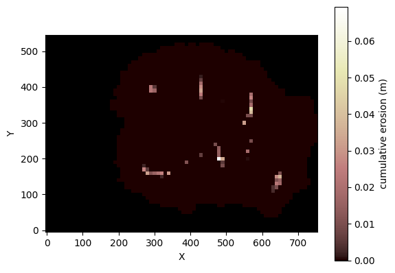
We can also inspect the cumulative erosion during the event by differencing the before and after terrain:

grid.imshow(starting_elev - elev, colorbar_label="cumulative erosion (m)")

Note that because this is a bumpy DEM, much of the erosion has occurred on (probably digital) steps in the channels. But we can see some erosion across the slopes as well.

DetachmentLtdErosion

This component is similar to DepthSlopeProductErosion except that it calculates erosion rate from discharge and slope rather than depth and slope. The vertical incision rate, \(I\) (equivalent to \(E\) in the above; here we are following the notation in the component’s documentation) is:

\[I = K Q^m S^n - I_c\]

where \(K\) is an erodibility coefficient (with dimensions of velocity per discharge\(^m\); specified by parameter K_sp), \(Q\) is volumetric discharge, \(I_c\) is a threshold with dimensions of velocity, and \(m\) and \(n\) are exponents. (In the erosion literature, the exponents are sometimes treated as empirical parameters, and sometimes set to particular values on theoretical grounds; here we’ll just set them to unity.)

The component uses the fields surface_water__discharge and topographic__slope for \(Q\) and \(S\), respectively. The component will modify the topographic__elevation field accordingly. If the user wishes to apply material uplift relative to baselevel, an uplift_rate parameter can be passed on initialization.

Here are the header and constructor docstrings:

from landlab.components import DetachmentLtdErosion

print(DetachmentLtdErosion.__doc__)

Simulate detachment limited sediment transport.

    Landlab component that simulates detachment limited sediment transport is more
    general than the stream power component. Doesn't require the upstream node
    order, links to flow receiver and flow receiver fields. Instead, takes in
    the discharge values on NODES calculated by the OverlandFlow class and
    erodes the landscape in response to the output discharge.

    As of right now, this component relies on the OverlandFlow component
    for stability. There are no stability criteria implemented in this class.
    To ensure model stability, use StreamPowerEroder or FastscapeEroder
    components instead.

    .. codeauthor:: Jordan Adams

    Examples
    --------
    >>> import numpy as np
    >>> from landlab import RasterModelGrid
    >>> from landlab.components import DetachmentLtdErosion

    Create a grid on which to calculate detachment ltd sediment transport.

    >>> grid = RasterModelGrid((4, 5))

    The grid will need some data to provide the detachment limited sediment
    transport component. To check the names of the fields that provide input to
    the detachment ltd transport component, use the *input_var_names* class
    property.

    Create fields of data for each of these input variables.

    >>> grid.at_node["topographic__elevation"] = [
    ...     [0.0, 0.0, 0.0, 0.0, 0.0],
    ...     [1.0, 1.0, 1.0, 1.0, 1.0],
    ...     [2.0, 2.0, 2.0, 2.0, 2.0],
    ...     [3.0, 3.0, 3.0, 3.0, 3.0],
    ... ]

    Using the set topography, now we will calculate slopes on all nodes.

    >>> grid.at_node["topographic__slope"] = [
    ...     [0.0, 0.0, 0.0, 0.0, 0.0],
    ...     [0.70710678, 1.0, 1.0, 1.0, 0.70710678],
    ...     [0.70710678, 1.0, 1.0, 1.0, 0.70710678],
    ...     [0.70710678, 1.0, 1.0, 1.0, 0.70710678],
    ... ]


    Now we will arbitrarily add water discharge to each node for simplicity.

    >>> grid.at_node["surface_water__discharge"] = [
    ...     [30.0, 30.0, 30.0, 30.0, 30.0],
    ...     [20.0, 20.0, 20.0, 20.0, 20.0],
    ...     [10.0, 10.0, 10.0, 10.0, 10.0],
    ...     [5.0, 5.0, 5.0, 5.0, 5.0],
    ... ]

    Instantiate the `DetachmentLtdErosion` component to work on this grid, and
    run it. In this simple case, we need to pass it a time step ('dt')

    >>> dt = 10.0
    >>> dle = DetachmentLtdErosion(grid)
    >>> dle.run_one_step(dt=dt)

    After calculating the erosion rate, the elevation field is updated in the
    grid. Use the *output_var_names* property to see the names of the fields that
    have been changed.

    >>> dle.output_var_names
    ('topographic__elevation',)

    The `topographic__elevation` field is defined at nodes.

    >>> dle.var_loc("topographic__elevation")
    'node'


    Now we test to see how the topography changed as a function of the erosion
    rate.

    >>> grid.at_node["topographic__elevation"].reshape(grid.shape)
    array([[0.        , 0.        , 0.        , 0.        , 0.        ],
           [0.99936754, 0.99910557, 0.99910557, 0.99910557, 0.99936754],
           [1.99955279, 1.99936754, 1.99936754, 1.99936754, 1.99955279],
           [2.99968377, 2.99955279, 2.99955279, 2.99955279, 2.99968377]])

    References
    ----------
    **Required Software Citation(s) Specific to this Component**

    None Listed

    **Additional References**

    Howard, A. (1994). A detachment-limited model of drainage basin evolution. Water
    Resources Research  30(7), 2261-2285. https://dx.doi.org/10.1029/94wr00757

print(DetachmentLtdErosion.__init__.__doc__)

Calculate detachment limited erosion rate on nodes.

        Landlab component that generalizes the detachment limited erosion
        equation, primarily to be coupled to the the Landlab OverlandFlow
        component.

        This component adjusts topographic elevation.

        Parameters
        ----------
        grid : RasterModelGrid
            A landlab grid.
        K_sp : float, optional
            K in the stream power equation (units vary with other parameters -
            if used with the de Almeida equation it is paramount to make sure
            the time component is set to *seconds*, not *years*!)
        m_sp : float, optional
            Stream power exponent, power on discharge
        n_sp : float, optional
            Stream power exponent, power on slope
        uplift_rate : float, optional
            changes in topographic elevation due to tectonic uplift
        entrainment_threshold : float, optional
            threshold for sediment movement
        slope : str
            Field name of an at-node field that contains the slope.

The example below uses the same approach as the previous example, but now using DetachmentLtdErosion. Note that the value for parameter \(K\) (K_sp) is just a guess. Use of exponents \(m=n=1\) implies the use of total stream power.

# Process parameters
n = 0.1  # roughness coefficient, (s/m^(1/3))
dep_exp = 5.0 / 3.0  # depth exponent
R = 72.0  # runoff rate, mm/hr
K_sp = 1.0e-7  # erosion coefficient (m/s)/(m3/s)
m_sp = 1.0  # discharge exponent
n_sp = 1.0  # slope exponent
I_c = 0.0001  # erosion threshold, m/s

# Run-control parameters
rain_duration = 240.0  # duration of rainfall, s
run_time = 480.0  # duration of run, s
dt = 10.0  # time-step size, s
dem_filename = "../hugo_site_filled.asc"

# Derived parameters
num_steps = int(run_time / dt)

# set up arrays to hold discharge and time
time_since_storm_start = np.arange(0.0, dt * (2 * num_steps + 1), dt)
discharge = np.zeros(2 * num_steps + 1)

# Read the DEM file as a grid with a 'topographic__elevation' field
with open(dem_filename) as fp:
    grid = esri_ascii.load(fp, name="topographic__elevation", at="node")
elev = grid.at_node["topographic__elevation"] = elev

# Configure the boundaries: valid right-edge nodes will be open;
# all NODATA (= -9999) nodes will be closed.
grid.status_at_node[grid.nodes_at_right_edge] = grid.BC_NODE_IS_FIXED_VALUE
grid.status_at_node[np.isclose(elev, -9999.0)] = grid.BC_NODE_IS_CLOSED

slp_mag, slp_x, slp_y = slope_magnitude_at_node(grid, elev)
grid.add_field("topographic__slope", slp_mag, at="node", clobber=True)

array([0., 0., 0., ..., 0., 0., 0.])

# Instantiate the component
olflow = KinwaveImplicitOverlandFlow(
    grid, runoff_rate=R, roughness=n, depth_exp=dep_exp
)

dle = DetachmentLtdErosion(
    grid, K_sp=K_sp, m_sp=m_sp, n_sp=n_sp, entrainment_threshold=I_c
)

starting_elev = elev.copy()

for i in trange(num_steps):
    olflow.run_one_step(dt)
    dle.run_one_step(dt)
    slp_mag[:], slp_x, slp_y = slope_magnitude_at_node(grid, elev)

grid.imshow(starting_elev - elev, colorbar_label="cumulative erosion (m)")

---

Generated by nbsphinx from a Jupyter notebook.