Note

This page was generated from a jupyter notebook.

Using the Landlab 1D flexure component

In this example we will: * create a Landlab component that solves the (1D) flexure equation * apply a point load * run the component * plot some output * apply a distributed load

(Note that this tutorial uses the one-dimensional flexure component, Flexure1D. A separate tutorial notebook, “lots_of_loads”, explores the two-dimensional elastic flexure component Flexure.)

A bit of magic so that we can plot within this notebook.

# %matplotlib inline
import matplotlib.pyplot as plt
import numpy as np

Create the grid

We are going to build a uniform rectilinear grid with a node spacing of 100 km in the y-direction and 10 km in the x-direction on which we will solve the flexure equation.

First we need to import RasterModelGrid.

from landlab import RasterModelGrid

Create a rectilinear grid with a spacing of 100 km between rows and 10 km between columns. The numbers of rows and columms are provided as a tuple of (n_rows, n_cols), in the same manner as similar numpy functions. The spacing is also a tuple, (dy, dx).

grid = RasterModelGrid((3, 800), xy_spacing=(100e3, 10e3))

grid.dy, grid.dx

(np.float64(10000.0), np.float64(100000.0))

Create the component

Now we create the flexure component and tell it to use our newly created grid. First, though, we’ll examine the Flexure component a bit.

from landlab.components import Flexure1D

The Flexure1D component, as with most landlab components, will require our grid to have some data that it will use. We can get the names of these data fields with the input_var_names attribute of the component class.

Flexure1D.input_var_names

('lithosphere__increment_of_overlying_pressure',)

We see that flexure uses just one data field: the change in lithospheric loading. Landlab component classes can provide additional information about each of these fields. For instance, to see the units for a field, use the var_units method.

Flexure1D.var_units("lithosphere__increment_of_overlying_pressure")

'Pa'

To print a more detailed description of a field, use var_help.

Flexure1D.var_help("lithosphere__increment_of_overlying_pressure")

name: lithosphere__increment_of_overlying_pressure
description:
  Applied pressure to the lithosphere over a time step
units: Pa
unit agnostic: True
at: node
intent: in

What about the data that Flexure1D provides? Use the output_var_names attribute.

Flexure1D.output_var_names

('lithosphere_surface__increment_of_elevation',)

Flexure1D.var_help("lithosphere_surface__increment_of_elevation")

name: lithosphere_surface__increment_of_elevation
description:
  The change in elevation of the top of the lithosphere (the land
  surface) in one timestep
units: m
unit agnostic: True
at: node
intent: out

Now that we understand the component a little more, create it using our grid.

grid.add_zeros("lithosphere__increment_of_overlying_pressure", at="node")

flex = Flexure1D(grid, method="flexure")

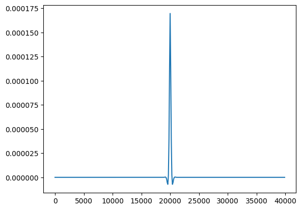
Add a point load

First we’ll add just a single point load to the grid. We need to call the update method of the component to calculate the resulting deflection (if we don’t run update the deflections would still be all zeros).

Use the load_at_node attribute of Flexure1D to set the loads. Notice that load_at_node has the same shape as the grid. Likewise, x_at_node and dz_at_node also reshaped.

flex.load_at_node[1, 200] = 1e6
flex.update()
plt.plot(flex.x_at_node[1, :400] / 1000.0, flex.dz_at_node[1, :400])

[<matplotlib.lines.Line2D at 0x10b9ec530>]

Before we make any changes, reset the deflections to zero.

flex.dz_at_node[:] = 0.0

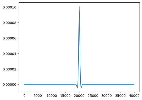
Now we will double the effective elastic thickness but keep the same point load. Notice that, as expected, the deflections are more spread out.

flex.eet *= 2.0
flex.update()
plt.plot(flex.x_at_node[1, :400] / 1000.0, flex.dz_at_node[1, :400])

[<matplotlib.lines.Line2D at 0x10c2338f0>]

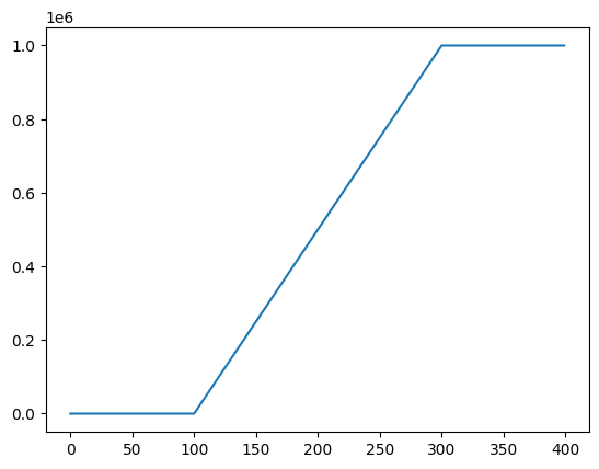
Add some loading

We will now add a distributed load. As we saw above, for this component, the name of the attribute that holds the applied loads is load_at_node. For this example we create a loading that increases linearly of the center portion of the grid until some maximum. This could by thought of as the water load following a sea-level rise over a (linear) continental shelf.

flex.load_at_node[1, :100] = 0.0
flex.load_at_node[1, 100:300] = np.arange(200) * 1e6 / 200.0
flex.load_at_node[1, 300:] = 1e6

plt.plot(flex.load_at_node[1, :400])

[<matplotlib.lines.Line2D at 0x10c2d2990>]

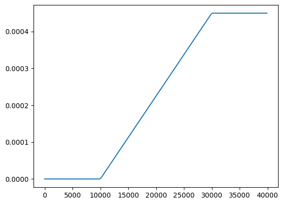
Update the component to solve for deflection

Clear the current deflections, and run update to get the new deflections.

flex.dz_at_node[:] = 0.0
flex.update()

plt.plot(flex.x_at_node[1, :400] / 1000.0, flex.dz_at_node[1, :400])

[<matplotlib.lines.Line2D at 0x10c343ec0>]

Exercise: try maintaining the same loading distribution but double the effective elastic thickness.

---

Generated by nbsphinx from a Jupyter notebook.