Note

This page was generated from a jupyter notebook.

How to do “D4” pit-filling on a digital elevation model (DEM)

(Greg Tucker, July 2021)

Digital elevation models (DEMs) often contain “pits”: cells or groups of cells that represent depressions, and are surrounded by higher-elevation cells. Sometimes these pits represent real landscape features, such as sinkholes in a karst landscape, or “pools” along a dry river channel. In other cases, they are artifacts of errors in the original data or of data processing. Sometimes they reflect a truncated representation of elevation values. For example, some DEMs use integer values to represent elevation in meters. Adjacent cells that differ by less than a meter in elevation can register as having exactly the same elevation in an integer DEM, making the drainage pathways in ambiguous.

For some overland flow models, depressions in a DEM are no problem: water will simply pool in the depressions and overspill when the depression is full. But overland flow models that use the kinematic wave approximation, in which the ground-surface slope is used as a proxy for the hydraulic energy slope, can not do this. Therefore, 2D overland flow models, like the Landlab components KinwaveOverlandFlowModel and KinwaveImplicitOverlandFlow, require a DEM that has had its pits and flat areas digitally removed before they can be run reliably.

This tutorial describes how to do this using Landlab’s flow-routing and pit-filling components.

First, some imports:

from landlab.components import FlowAccumulator
from landlab.io import esri_ascii

Read the un-filled DEM, which happens to be in Arc/Info ASCII Grid format (a.k.a., ESRI ASCII). We will use the set_watershed_boundary_condition function to set all nodes with an elevation value equal to a “no data” code (default -9999) to closed boundaries, and any nodes with valid elevation values that lie on the grid’s perimeter to open (fixed value) boundaries. You can learn more about the raster version of this handy function here.

# Read a small DEM
with open("hugo_site.asc") as fp:
    grid = esri_ascii.load(fp, name="topographic__elevation", at="node")

# This sets nodes with a no-data code (default -9999) to closed boundary status
# (For a perimeter node to be considered )
grid.set_watershed_boundary_condition(grid.at_node["topographic__elevation"])

Having read the DEM and set its boundary conditions, we now instantiate and run FlowAccumulator. We will tell it to use “D4” routing, which is indicated by the parameter choice flow_director = FlowDirectorSteepest. (Note that the term “steepest” means “choose the steepest drop among all directly adjacent nodes”. In a RasterModelGrid, there are normally four neighboring nodes, and so when FlowDirectorSteepest is applied to a raster grid, it does ‘D4’ routing. When it is applied to a hex grid, for example, it chooses among six possible directions. This variation in the number of potential directions depending on grid type is why it this particular flow-direction method is called “steepest” rather than “D4”. For more on this, see the tutorials the_FlowDirectors and compare_FlowDirectors.)

First, we will run the flow accumulator without any depression handling, in order to visualize the drainage in this case:

fa_no_fill = FlowAccumulator(grid, flow_director="FlowDirectorSteepest")
fa_no_fill.run_one_step()

grid.imshow("drainage_area", colorbar_label="Drainage area (m2)")

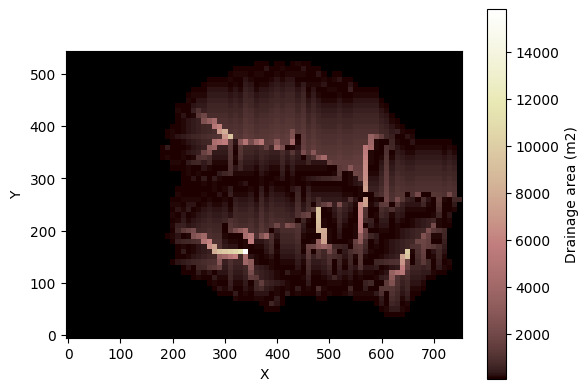
Notice that there are interruptions in the drainage patterns: places where drainage area abruptly drops in the downstream direction. These spots represent drainages that terminate in pits.

Now we’ll repeat the process, but this time we will also tell the FlowAccumulator to use the LakeMapperBarnes component for depression handling. (Note that we could run LakeMapperBarnes separately, but because depression handling and flow accumulation work together, the FlowAccumulator provides a way to directly “embed” a depression handler and its arguments, which is the approach used here; you can learn more about this in the tutorial the_FlowAccumulator.) We can examine the parameters of LakeMapperBarnes:

from landlab.components import LakeMapperBarnes

print(LakeMapperBarnes.__init__.__doc__)

Initialize the component.

        Parameters
        ----------
        grid : ModelGrid
            A grid.
        surface : field name at node or array of length node
            The surface to direct flow across.
        method : {'Steepest', 'D8'}
            Whether or not to recognise diagonals as valid flow paths, if a raster.
            Otherwise, no effect.
        fill_flat : bool
            If True, pits will be filled to perfectly horizontal. If False, the new
            surface will be slightly inclined to give steepest descent flow paths
            to the outlet.
        fill_surface : bool
            Sets the field or array to fill. If fill_surface is surface, this
            operation occurs in place, and is faster.
            Note that the component will overwrite fill_surface if it exists; to
            supply an existing water level to it, supply that water level field as
            surface, not fill_surface.
        redirect_flow_steepest_descent : bool
            If True, the component outputs modified versions of the
            'flow__receiver_node', 'flow__link_to_receiver_node',
            'flow__sink_flag', and 'topographic__steepest_slope' fields. These
            are the fields output by the FlowDirector components, so set to
            True if you wish to pass this LakeFiller to the FlowAccumulator,
            or if you wish to work directly with the new, correct flow directions
            and slopes without rerunning these components on your new surface.
            Ensure the necessary fields already exist, and have already been
            calculated by a FlowDirector! This also means you need to instantiate
            your FlowDirector **before** you instantiate the LakeMapperBarnes.
            Note that the new topographic__steepest_slope will always be set to
            zero, even if fill_flat=False (i.e., there is actually a miniscule
            gradient on the new topography, which gets ignored).
        reaccumulate_flow : bool
            If True, and redirect_flow_steepest_descent is True, the run method
            will (re-)accumulate the flow after redirecting the flow. This means
            the 'drainage_area', 'surface_water__discharge',
            'flow__upstream_node_order', and the other various flow accumulation
            fields (see output field names) will now reflect the new drainage
            patterns without having to manually reaccumulate the discharge. If
            True but redirect_flow_steepest_descent is False, raises an
            ValueError.
        ignore_overfill : bool
            If True, suppresses the Error that would normally be raised during
            creation of a gentle incline on a fill surface (i.e., if not
            fill_flat). Typically this would happen on a synthetic DEM where more
            than one outlet is possible at the same elevation. If True, the
            was_there_overfill property can still be used to see if this has
            occurred.
        track_lakes : bool
            If True, the component permits a slight hit to performance in order to
            explicitly track which nodes have been filled, and to enable queries
            on that data in retrospect. Set to False to simply fill the surface
            and be done with it.

If we don’t wish to accept the built-in defaults, we can send any of these parameters as additional arguments to the FlowAccumulator constructor. For this application, we want:

• surface = topographic__elevation: use the topography (this is the default)

• method = 'Steepest': use D4 routing (the default)

• fill_flat = False: we want a slight slope assigned to otherwise flat areas

• fill_surface = 'topographic__elevation': fill the topography (the default)

• redirect_flow_steepest_descent = True: so we can plot the revised drainage

• reaccumulate_flow = True: so we can plot the revised drainage

fa = FlowAccumulator(
    grid,
    flow_director="FlowDirectorSteepest",
    depression_finder="LakeMapperBarnes",
    surface="topographic__elevation",
    method="Steepest",
    fill_flat=False,
    fill_surface="topographic__elevation",
    redirect_flow_steepest_descent=True,
    reaccumulate_flow=True,
)

original_elev = grid.at_node[
    "topographic__elevation"
].copy()  # keep a copy of the original
fa.run_one_step()
grid.imshow("drainage_area", colorbar_label="Drainage area (m2)")

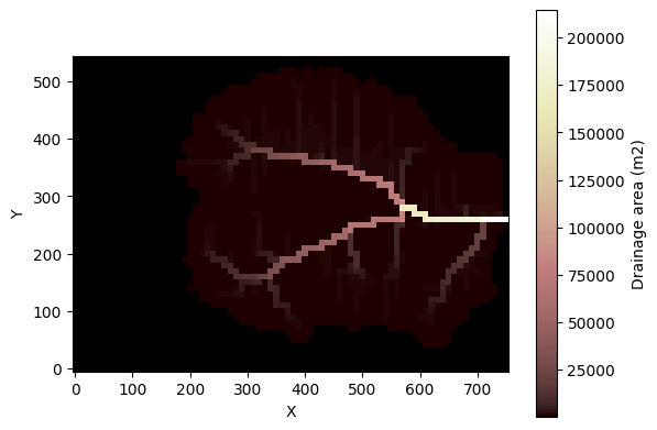
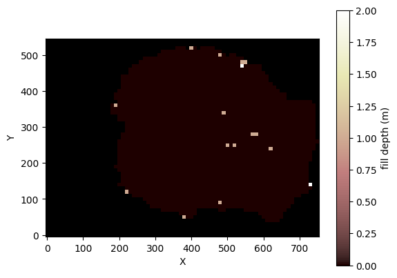
Now we have a continuous drainage system that passes smoothly over the now-filled pits. Drainage from every cell in the watershed can reach the outlet. By plotting the difference between the original and modified topography, we can inspect the depth and spatial patterns of pit filling:

grid.imshow(
    grid.at_node["topographic__elevation"] - original_elev,
    colorbar_label="fill depth (m)",
)

---

Generated by nbsphinx from a Jupyter notebook.