Note

This page was generated from a jupyter notebook.

2D Surface Water Flow component

River Flow Dynamics Simulation with Landlab

---

For more Landlab tutorials, click here: https://landlab.csdms.io/tutorials/

---

Overview

This notebook demonstrate the usage of the river flow dynamics Landlab component. The component runs a semi-implicit, semi-Lagrangian finite-volume approximation to the depth-averaged 2D shallow-water equations of Casulli and Cheng (1992) and related work.

This notebook demonstrates how to simulate river flow dynamics using the Landlab library, implementing the semi-implicit, semi-Lagrangian finite-volume approximation of the depth-averaged shallow water equations (Casulli and Cheng, 1992).

Setup and Imports

Import the needed libraries:

import matplotlib.pyplot as plt
import numpy as np

from landlab import RasterModelGrid
from landlab.components import RiverFlowDynamics  # Note: Using updated CamelCase naming
from landlab.plot.imshow import imshow_grid

Create Grid and Set Initial Conditions

First, let’s create a rectangular grid for our flow dynamics calculations:

nRows = 20
nCols = 60
cellSize = 0.1

Creating the grid

grid = RasterModelGrid((nRows, nCols), xy_spacing=(cellSize, cellSize))

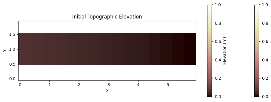
Setting up the initial topographic elevation

te = grid.add_zeros("topographic__elevation", at="node")
te += 0.059 - 0.01 * grid.x_of_node
te[grid.y_of_node > 1.5] = 1.0
te[grid.y_of_node < 0.5] = 1.0

Visualizing the initial topography

plt.figure(figsize=(12, 4))
imshow_grid(grid, "topographic__elevation")
plt.title("Initial Topographic Elevation")
plt.colorbar(label="Elevation (m)")
plt.show()

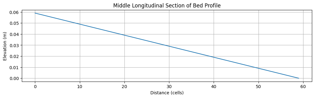
Visualizing the middle bed profile

middleBedProfile = np.reshape(te, (nRows, nCols))[10, :]
plt.figure(figsize=(12, 3))
plt.plot(middleBedProfile)
plt.title("Middle Longitudinal Section of Bed Profile")
plt.xlabel("Distance (cells)")
plt.ylabel("Elevation (m)")
plt.grid(True)
plt.show()

Initializing Required Fields

Create water depth field (initially empty channel)

h = grid.add_zeros("surface_water__depth", at="node")

Create velocity field (initially zero)

vel = grid.add_zeros("surface_water__velocity", at="link")

Calculate initial water surface elevation

wse = grid.add_zeros("surface_water__elevation", at="node")
wse += h + te

Setting up the boundary conditions

fixed_entry_nodes = np.arange(300, 910, 60)
fixed_entry_links = grid.links_at_node[fixed_entry_nodes][:, 0]

Set fixed values for entry nodes/links

entry_nodes_h_values = np.full(11, 0.5)  # 0.5m water depth
entry_links_vel_values = np.full(11, 0.45)  # 0.45 m/s velocity

Run Simulation

Initialize the RiverFlowDynamics component

rfd = RiverFlowDynamics(
    grid,
    dt=0.1,
    mannings_n=0.012,
    fixed_entry_nodes=fixed_entry_nodes,
    fixed_entry_links=fixed_entry_links,
    entry_nodes_h_values=entry_nodes_h_values,
    entry_links_vel_values=entry_links_vel_values,
)

Run the simulation for 100 timesteps (10 seconds)

n_timesteps = 100
for timestep in range(n_timesteps):
    rfd.run_one_step()

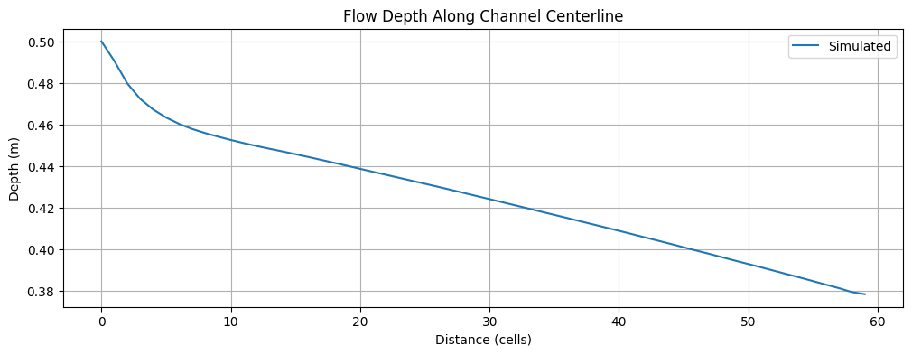
Analyze Results

Get flow depth along center of channel

flow_depth = np.reshape(grid["node"]["surface_water__depth"], (nRows, nCols))[10, :]

Plot flow depth

plt.figure(figsize=(12, 4))
plt.plot(flow_depth, label="Simulated")
plt.title("Flow Depth Along Channel Centerline")
plt.xlabel("Distance (cells)")
plt.ylabel("Depth (m)")
plt.grid(True)
plt.legend()
plt.show()

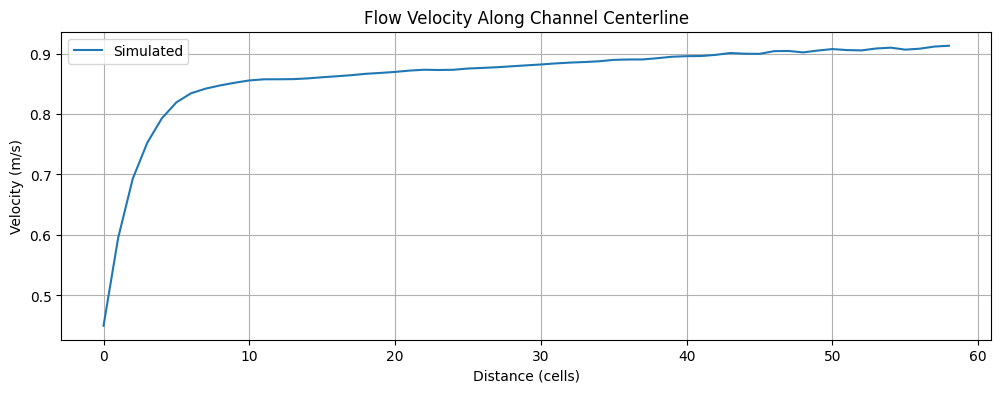
Get and plot velocity along center of channel

linksAtCenter = grid.links_at_node[np.array(np.arange(600, 660))][:-1, 0]
flow_velocity = grid["link"]["surface_water__velocity"][linksAtCenter]

plt.figure(figsize=(12, 4))
plt.plot(flow_velocity, label="Simulated")
plt.title("Flow Velocity Along Channel Centerline")
plt.xlabel("Distance (cells)")
plt.ylabel("Velocity (m/s)")
plt.grid(True)
plt.legend()
plt.show()

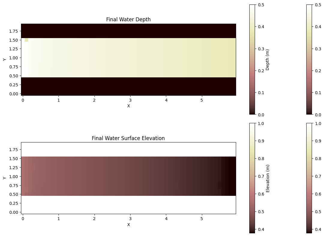
Visualization of Final State

Create a figure with two subplots and then let’s plot final water depth

fig, (ax1, ax2) = plt.subplots(2, 1, figsize=(12, 8))

# Plot final water depth
plt.subplot(2, 1, 1)
im1 = imshow_grid(grid, "surface_water__depth")
plt.title("Final Water Depth")
plt.colorbar(label="Depth (m)")

# Plot final water surface elevation
plt.subplot(2, 1, 2)
im2 = imshow_grid(grid, "surface_water__elevation")
plt.title("Final Water Surface Elevation")
plt.colorbar(label="Elevation (m)")

plt.tight_layout()
plt.show()

###	And that’s it!
Nic	e work completing this tutorial. You know now how to use the Ri verFlowDynamics Landlab component to run your own simulations :)

Click here for more Landlab tutorials

---

Generated by nbsphinx from a Jupyter notebook.